Purpose
Biology’s first big data era — defined by the opportunistic, random accumulation of sequences and structures — is due for an overhaul. While biological foundation models (BFMs) represent the zenith of this era, their utility will always be hamstrung by the inherent non-independence of biological data. Massive increases in data volume don’t yield proportional increases in unique information. We argue that the next era of biology must be prospective rather than retrospective. We show that even a simple Bayesian framework can move us beyond the "bitter lesson" of brute-force scaling and instead treat biological measurement as a strategic act of inference. There’s no excuse to gather data blindly; biology must become prospective.
This pub is intended for computational biologists, machine learning researchers, and anyone modelling the complexities of life. It’s especially relevant for funders, decision makers, and researchers invested in large-scale biological data collection efforts and the development of biological foundation models.
Background
With origins in the molecular biology revolution of the 1970s, biology’s first big data era gained momentum about 25 years ago with the widespread availability of genome sequencing. Public databases have grown exponentially ever since 1. Exploratory analyses of high-dimensional datasets have become commonplace, and new data-oriented disciplines — such as bioinformatics, genomics (and -omics in general), computational biology, and systems biology — have emerged. Biological research has shifted mainly from being hypothesis- to data-driven 2–3.
Biological foundation models (BFMs) sit at the zenith of this era. As large-scale machine learning systems, BFMs leverage the avalanche of biological data generated over the past quarter-century: molecular sequences (e.g., DNA, RNA, proteins), cellular and tissue-level images, high-dimensional omics measurements (e.g., transcriptomics, proteomics, metabolomics), and even entire genomes. BFMs are designed as general-purpose statistical tools. They're extensively pre-trained to capture broad, transferable representations that can adapt to diverse applications. Cell-based BFMs (e.g., virtual cell models), for instance, may identify therapeutic targets, engineer synthetic pathways, or infer emergent cellular properties 4. Sequence-based BFMs, including protein/genomic language models (pLMs and gLMs), might generate novel sequences, annotate them, or explore complex fitness landscapes 5. What’s more, the internal representations learned by BFMs may reflect deep principles about the organization of life 6.
BFMs are a fitting culmination of biology’s first big data era. They may well also be the harbinger of its end. Like all statistical models, the utility of BFMs depends not only on the volume of data but also on its composition 7. The public databases that supply most training material — e.g., UniRef 8, the Protein Data Bank 9, MGnify 10, RefSeq 11, and GenBank 12 — have grown opportunistically, reflecting the distributed and often biased sampling priorities of the biological community. Unsurprisingly, data imbalances abound 13. Around 40% of structures in the Protein Data Bank are human 9, 14, UniRef is dominated by a few bacterial phyla 14, and five species account for over 65% of the Sequence Read Archive 13.
These imbalances matter. Training data composition shapes what BFMs can learn: high-frequency sequences disproportionately influence model predictions and generations 15–16. Latent correlations between training, validation, and test data can lead to data leakage, allowing models to reproduce patterns rather than generalize them. Leakage has been documented across various modalities — pLMs 17, gLMs 18–19, neuroimaging 20, and medical imaging foundation models 21. When data points are evolutionarily or structurally related, models can "cheat" by exploiting redundancy, inflating apparent performance while leaving underlying biases uncorrected. Statistical models that ignore these dependencies risk pseudoreplication — the treatment of correlated measurements as independent observations 22–23.
Pseudoreplication can have various undesirable consequences, and tools for mitigating it in BFMs are in their infancy. For example, biases observed in pLMs and gLMs often arise from latent evolutionary relationships among training sequences 19. It’s possible that phylogenetic methods can help identify and correct these relationships. Some recent models — such as Phyla 24, MSA Pairformer 25, and STAR-GPN 26 — explicitly incorporate phylogenetic information to achieve strong performance with comparatively few parameters. Another approach is to prune non-independent data before training, although this often reduces the effective sample size dramatically 14, 19. This helps explain the recent plateau in performance for many pLMs trained on UniRef50 27 — a potential "peak data" scenario in which models have already absorbed most of the unique information available.
In general, the prevailing response to these challenges has been to scale further: gather more data, train larger models, and embrace the "bitter lesson" that compute and scale always win 7, 28. BaseData 13 and OpenGenome2 28 each contain nearly ten trillion genomic tokens — orders of magnitude larger than previous public resources. The Logan database lists over 100 billion proteins, a 30-fold increase over UniRef50 29. The Earth BioGenome Project aims to sequence all eukaryotic species 30. While additional resources will undoubtedly expand the capabilities of BFMs, all gains aren't created equal.
Like their predecessors, these massive datasets are also products of random, opportunistic sampling. OpenGenome2 and Logan are derived from public repositories 28–29, whereas BaseData expands through large-scale environmental sequencing 13. Each new data source introduces new information. They also introduce redundancy. Because of evolutionary nonindependence, statistical power doesn't scale linearly with sample size. A 30-fold increase in data volume doesn't yield 30-fold increases in unique information. Indeed, once redundancy is accounted for, effective sample sizes shrink drastically — sometimes to a fraction of the nominal database size. Non-independence also exists on a continuum; nearly every protein family shows some degree of correlation 19.
Consequently, for every sequencing dollar spent under random sampling, some fraction inevitably funds the recollection of information we already possess — information that's duplicated at molecular, structural, or evolutionary levels. We seldom know how much redundancy we're adding, where it occurs, or how it biases downstream models. What’s more, our understanding of the limitations of BFMs has been entirely retrospective. We typically train a massive model, celebrate its scale, and only then perform forensic audits to discover what it actually learned. Worse, we still lack a precise estimate of how much data — or which model architectures — will be required for BFMs to truly generalize across biology. From a taxonomic standpoint, we have only begun to scratch the surface: reference genomes exist for roughly 1% of eukaryotic species 30, and billions of prokaryotic lineages remain undiscovered. If our goal is to uncover general principles of life, the gap remains daunting.
So how should biology move forward? Passive, random data accumulation will no longer suffice. And just because the cost of generating, storing, and analyzing data decreases over time, we shouldn’t indiscriminately capture it. Nonindependence ensures that the effective number of unique biological dimensions grows far more slowly than the number of measurements. Exclusively retrospective analyses will also be insufficient as data, computation, and model size all scale. Biology’s next era must be prospective: linking what we already know to what new observations can teach us — a way to quantify novelty, redundancy, and diminishing returns as data accumulate and models update.
Fortunately, transitioning from blind accumulation need not require Herculean efforts. Many frameworks already exist to help guide the collection of information. Even basic, if imperfect, application of these frameworks would benefit comparative data collection. What’s more, these frameworks are flexible. As long as the user can capture their data via a distribution and define a reasonable measurement goal (more on this below), many of these approaches can be applied to data in an agnostic manner. The utility of new data, whether RNA expression levels, genome sequences, or medical images, can be assessed within these frameworks, enabling comprehensive analysis of a broad range of biological data.
In what follows, we outline a basic framework for Bayesian collection of comparative biological data. Our goal is to highlight how we might transition from random, scale-driven data collection to an adaptive, inference-driven process — one that treats biological measurement as an act of learning rather than mere accumulation. To be more explicit, if you’ve ever wondered about the source, composition, or structure of data that'll best inform your downstream purpose (more bang for your data collection buck), this is for you.
The idea
Bayesian reasoning formalizes learning from evidence as an iterative process: prior beliefs are updated by new data to yield a posterior distribution that captures remaining uncertainty. This framing is particularly natural for biological data, which are heterogeneous, hierarchical, and non‑independent. In what follows, we interleave key Bayesian concepts with a concrete case study — the AlphaFold Database (AFDB) — to show how Bayesian thinking can guide not only retrospective analysis, but prospective data collection.
The AFDB contains over 214 million predicted protein structures 31. Recent work has aggregated these structures into ~2.3 million clusters, each representing a putative structural or functional class 32. These structures span organisms across the tree of life (ToL), yet the database is far from uniform 14. Previous analyses showed that a small number of bacterial taxa dominate the AFDB and tend to yield higher-confidence (pLDDT) predictions. At the same time, many other lineages — particularly across eukaryotes — remain sparsely sampled 14. Importantly, these disparities persist even after data balancing, suggesting that simple reweighting can't compensate for missing diversity 14. The problem isn't how to rebalance existing data, but where to collect new data.
This question — where would additional data provide the greatest return? — is naturally Bayesian. Answering it requires us to be explicit about (i) our prior knowledge, (ii) how new observations update that knowledge, and (iii) the specific quantity we want to optimize.
An initial decision concerns the unit of analysis. Should new data be counted as individual proteins, Foldseek clusters, environmental samples, or whole proteomes? Different choices imply different priors and different interpretations. Here, we focus on species‑level proteomes obtained through genome sequencing. Each new species is treated as a single experiment that updates our understanding of protein structural space.
Given this choice, each proteome can be represented as a discrete distribution over Foldseek clusters: the counts of proteins belonging to each of ~2 million clusters define a species‑specific "structural footprint." Aggregating these footprints across all previously sequenced species yields a natural prior — a Dirichlet distribution over protein clusters — that encodes our current beliefs about how protein structures are distributed across life.
When a new species is sequenced, its observed cluster footprint can be evaluated under this prior. In Bayesian terms, this is the likelihood: the probability of observing that particular distribution of clusters given our existing model. Updating the prior with this likelihood yields a posterior Dirichlet distribution that reflects how our beliefs about protein structural space have changed after incorporating the new proteome.
This framing emphasizes that not all new data are equally informative. A species whose proteome closely resembles those already sampled will induce only a slight shift in the posterior. In contrast, a species enriched for rare or novel clusters will substantially reshape it.
To formalize this intuition, we must specify our estimand — the quantity we aim to measure. Here, we define the estimand as the information provided by a new proteome. Operationally, this is captured by the Kullback–Leibler (KL) divergence between the prior and posterior Dirichlet distributions. We refer to this quantity as the information gain (IG).
Under this definition, IG is low when a proteome essentially reinforces existing beliefs and high when it introduces substantial novelty. Crucially, IG is conditional: it depends on the current prior, the unit of analysis, and the way data are incorporated.
Before quantifying information gain, it's useful to examine the global relationships among species‑level proteome fingerprints (Figure 1). Nonlinear embeddings of these distributions reveal broad taxonomic structure. Species cluster by domain — Eukaryotes, Archaea, and Bacteria — and, to a lesser extent, by kingdom (Figure 1). Two bacterial clades, Pseudomonadati and Bacillati, dominate the embedding, while eukaryotes separate into fungi/metazoa and viridiplantae (Figure 1). These patterns suggest that proteomes are neither independent nor redundant, and that taxonomy provides an informative — if imperfect — prior for estimating novelty.
Our first analysis asks: how much information do species from different taxa tend to contribute? For each phylum, we construct a prior that excludes that phylum and compute the IG for each of its species. This approach treats species as independent and ignores proteome size, making it a coarse, taxonomy‑only baseline that reflects minimal prior knowledge.
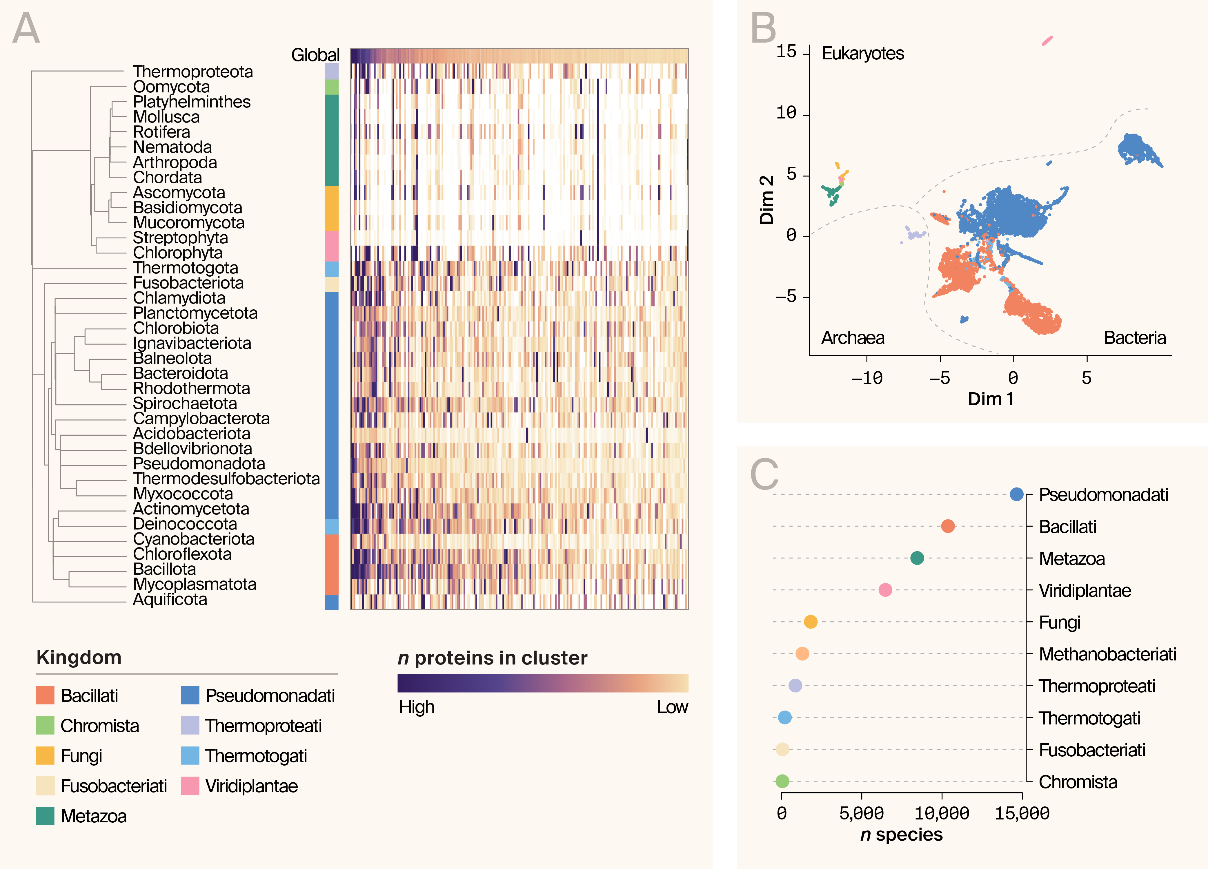
Figure 1. Overview of proteome variation in the AFDB.
(A) Example protein cluster "fingerprints" for major phyla. Protein number is indicated by the heatmap; more proteins in a cluster correspond to a darker color (white indicates no proteins in the cluster). Global totals are indicated by the top row. Included are the 500 largest AFDB structural clusters. Kingdoms are indicated by color to the left of the fingerprints.
(B) UMAP embedding of per-species AFDB fingerprints. Species are colored by kingdom.
(C) Distribution of species abundance in the dataset by kingdom.
Apparent domain‑level differences emerge (Figure 2). Eukaryotic phyla contribute substantially more information on average (mean IG = 4999 bits) than bacterial (523 bits) or archaeal phyla (166 bits). Streptophyta (land plants and green algae) exhibit the highest mean IG (IG = 11516 bits), while Aquificota rank lowest (IG = 2 bits). Eukaryotic phyla also show more consistent IG values within phyla, whereas bacterial phyla display much greater variability (p = 2 × 10⁻⁵; Kruskal–Wallis test on phylum-level coefficients of variation) (Figure 2). Taken at face value, this suggests that expanding eukaryotic — particularly plant — sampling could yield significant gains in protein structural novelty.
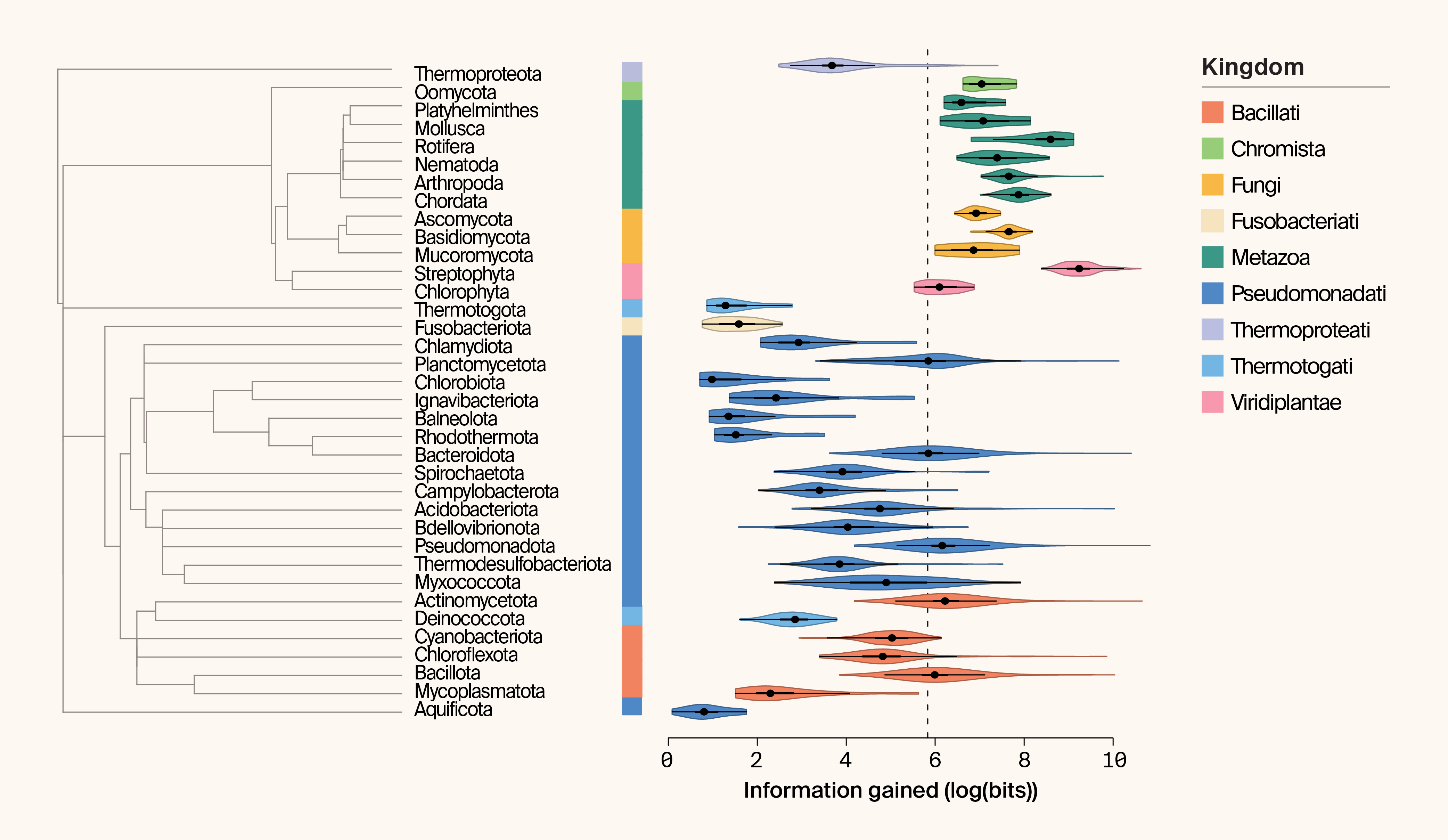
Figure 2. Phylogeny and paired violin plot of information gained (IG) per phylum.
IG is plotted as the logarithm of bits. The kingdom associated with each phylum is indicated by color. Median IG is indicated by the dashed line.
However, Bayesian estimates inherit the structure of the data-generating process. Eukaryotes tend to have much larger proteomes than prokaryotes, and IG is positively correlated with the number of proteins per species. More proteins naturally provide more opportunities to observe rare clusters. Indeed, most phyla follow a shared linear relationship between proteome size and IG (r = 0.53; Pearson correlation) (Figure 3).
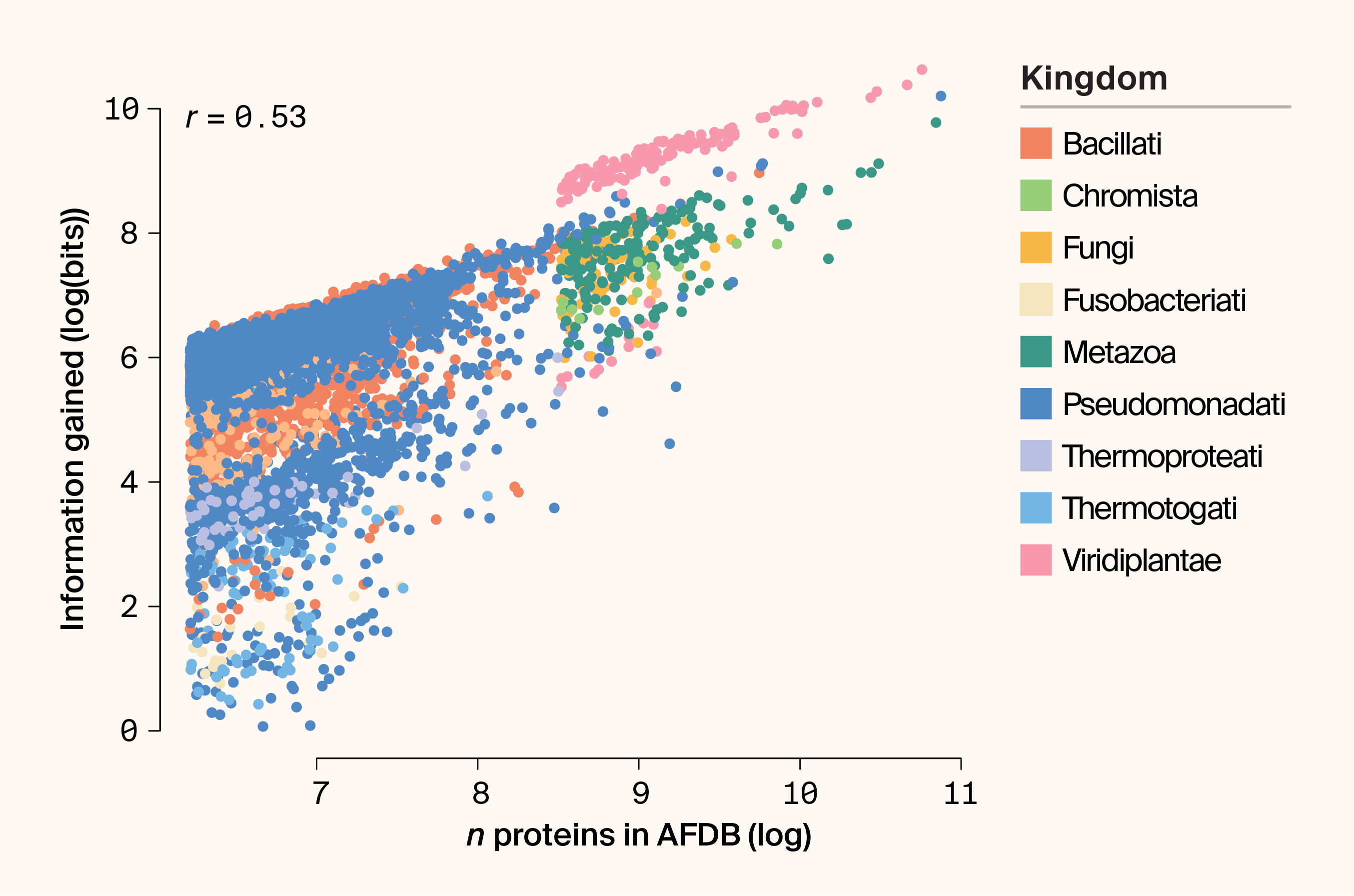
Figure 3. Scatter plot highlighting the relationship between proteome size and IG (plotted as the logarithm of bits).
The kingdom is indicated by color. r = Pearson’s correlation coefficient.
Viridiplantae nonetheless remain partial outliers, exhibiting higher IG than taxa with comparable proteome sizes. Extensive genome expansion and diversification in plant lineages may generate not only more proteins, but also more structurally diverse ones. From a Bayesian perspective, these proteomes induce huge posterior updates.
High information gain, however, doesn't necessarily imply efficient data collection. Large, repetitive genomes are costly to sequence and assemble. To account for this, we modify our likelihood function by holding sampling effort constant. Instead of whole proteomes, we randomly sample fixed‑size subsets (n = 100 proteins) from each species and compute IG for these subsamples, repeating the process to estimate average IG per n proteins.
This efficiency‑adjusted analysis reverses the earlier taxonomic patterns. Prokaryotic phyla now appear more information‑rich per sampled protein, with Mycoplasmatota ranking highest (Figure 4). All eukaryotic phyla fall below 0.2 bits of IG per 100 proteins (Figure 4). These results support the intuition that broad microbial sampling — such as metagenomics — can be an exceptionally efficient way to explore protein structural space.
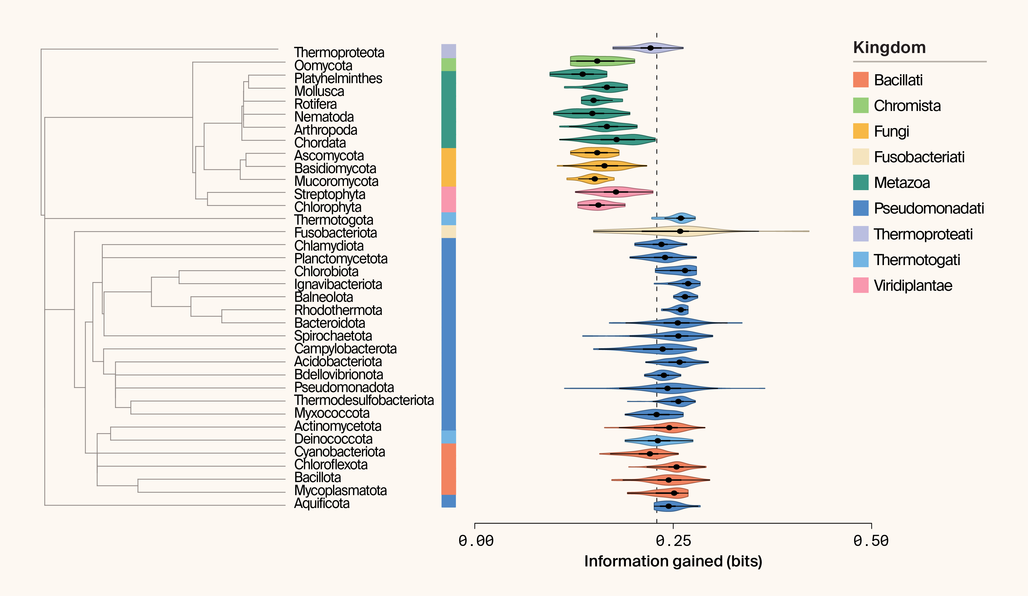
Figure 4. Phylogeny and paired violin plot of information gained (IG) per phylum using permutation-based sampling.
IG is plotted as the logarithm of bits. The kingdom associated with each phylum is indicated by color. Median IG is indicated by the dashed line.
Yet efficiency isn't the whole story. Under subsampling, IG variance is strongly negatively correlated with mean IG (r = −0.93; p = 4.95 × 10⁻²³) (Figure 5). Eukaryotes, while exhibiting lower mean IG per subsample, display much broader IG distributions: each random draw of 100 proteins is more distinct than comparable draws from prokaryotes. This highlights sampling density as a critical design parameter. Sparse sampling favors prokaryotes, while deeper sampling may allow large eukaryotic proteomes to continue yielding novelty.
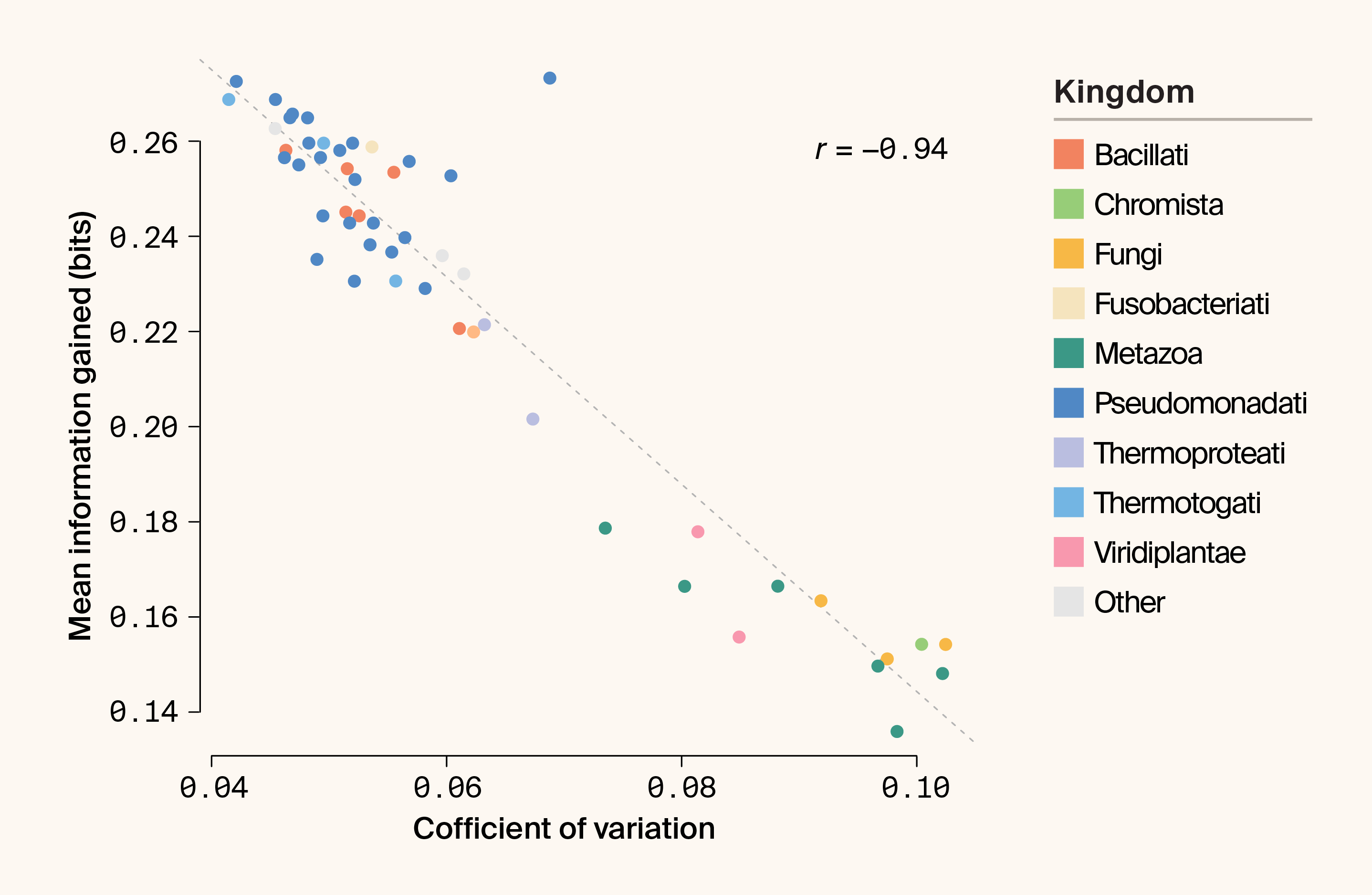
Figure 5. Scatter plot highlighting the relationship between the coefficient of variation (mean normalized variance) and mean IG (bits) under permutation-based sampling.
The kingdom is indicated by color. r = Pearson’s correlation coefficient.
Together, these examples underscore a central lesson: there's no single optimal dataset independent of context. The value of new data is conditional on our goals (the estimand), our current knowledge (the prior), and our constraints on sampling effort. If the aim is to maximize total structural novelty, eukaryotic genomes offer the highest ceiling. If efficiency per sequenced residue is paramount, microbial diversity provides the best return. By explicitly formalizing these trade-offs, a Bayesian framework empowers us to replace blind accumulation with strategic design. It moves the field from a retrospective audit of what's been learned to a prospective calculation of what should be measured next, ensuring that future data collection isn't just extensive, but intentional.
Conclusion
The end of biology’s first big data era isn't a signal to stop measuring; rather, it's a mandate to start measuring differently. As our examples demonstrate, the value of a biological dataset isn't intrinsic to its size (in terabytes) or breadth (in species count), but rather depends on the question being asked and the knowledge we already possess. Viewed through this lens, we see an inversion of the "bitter lesson" 33: efficient compute doesn’t require data to be simply abundant or diverse, but of high utility.
Transitioning to this prospective framework offers a path out of the plateau of diminishing returns. By explicitly modeling the dependencies between biological entities — whether they're evolutionary relationships between species or structural similarities between proteins — we can calculate the expected information gain of a proposed experiment before a single sample is sequenced. This effectively closes the loop between the "dry lab" of model training and the "wet lab" of data generation. Instead of being passive consumers of opportunistic databases, biological foundation models can become active participants in the scientific process, guiding experimentalists toward the "dark matter" of the biological universe — the rare, the divergent, and the truly novel.
Ultimately, the future of biological discovery won't belong to those who merely accumulate the largest haystacks or automate its brute force collection, but to those who develop the sharpest magnets for finding needles. By replacing random sampling with the precision of inference-driven design, we can ensure that the next era of biology is defined not just by how much we read, but by how much we learn.
Methods
The data we used are available on Zenodo.
Data acquisition and taxonomic classification
We obtained protein cluster data and associated metadata from Barrio-Hernández et al., 2023 32. Taxonomic information for each protein was retrieved by querying NCBI taxonomy identifiers using the taxonomizr (v0.11.1) 34 and taxizedb (v0.3.1) 35 R packages. To ensure robust statistical comparisons, we filtered the dataset to include only species with high-quality proteome representations: a minimum of 500 proteins for Bacteria and Archaea, and 5,000 proteins for Eukaryota. To allow permutation-based testing, we focused on phyla represented by at least 10 species within the filtered dataset.
A global phylogeny was derived from the Timetree of Life 36. To visualize broad evolutionary patterns, we simplified this tree to the phylum level using a custom subsampling approach: one representative species was randomly selected per phylum to serve as a tip label, and the tree was pruned accordingly using the ape package in R (v5.8) 37.
Characterizing taxonomic "fingerprints"
To define the protein landscape of different taxa, we calculated the distribution of protein cluster IDs for each species and phylum.
We identified the 500 most frequent protein clusters across the entire dataset to create a reference matrix. Distributions were normalized to the maximum cluster count within each taxon to allow for comparative visualization alongside the phylum-level phylogeny.
To explore high-dimensional structure in protein distributions, we identified the top 10,000 protein clusters. We performed principal component analysis (PCA) on the species-by-cluster frequency matrix, followed by uniform manifold approximation and projection (UMAP) 38 on the first 200 principal components to visualize taxonomic grouping in two dimensions.
Quantifying information gain
We employed a Bayesian framework to quantify the "novelty" or information content of a proteome relative to an established evolutionary background.
Example 1: For a focal phylum, a Dirichlet prior was established based on the protein cluster distributions of all other phyla in the dataset. The prior concentration parameters () were estimated using an empirical Bayes approach via the optimize function to maximize the Dirichlet-multinomial marginal likelihood.
We calculated the information gain (IG) for each species by measuring the Kullback–Leibler (KL) divergence between the prior and posterior distributions, both updated with the focal species' protein counts.
where is the sum of parameters and is the digamma function. Results were converted from nats to bits for interpretability.
Example 2: To control for the confounding effect of proteome size — where larger genomes naturally accumulate more information — we performed a permutation-based subsampling analysis. For each species, we randomly sampled 500 proteins and recalculated the IG over 10 iterations. This standardized metric allowed us to compare the "density" of novelty across diverse taxonomic groups regardless of total protein count.
Statistical differences in IG and its coefficient of variation across domains (Bacteria, Archaea, and Eukaryota) were assessed using Kruskal–Wallis tests. All visualizations, including phylogenetic heatmaps, UMAP plots, and violin plots of IG distributions, were generated in R using the arcadiathemeR (v0.1.0) 39 and vioplot (v0.5.0) 40.
The code for this work is available in this GitHub repository (DOI: 10.5281/zenodo.18475275).
AI usage
We used ChatGPT (GPT-5 Thinking) to help write code, help clarify and streamline text that we wrote, and suggest wording ideas and then chose which small phrases or sentence structure ideas to use. We also used Grammarly Business and Gemini (3.0 Pro) to suggest wording ideas and then chose which small phrases or sentence structure ideas to use.
Be the first to comment on this publication.