Purpose
Biological systems are organized hierarchically. Genetic variation is expressed through RNA, protein, cells, tissues, and ultimately, organisms. Yet we know surprisingly little about what this hierarchy does to the structure of phenotypic variation. Is information filtered and compressed as it moves toward the organism? Or does each layer add new axes of variation? Analyses rarely ask. It's common, for example, to analyze the same RNA-seq dataset with both linear methods, such as principal component analysis (PCA), and nonlinear methods, such as uniform manifold approximation and projection (UMAP) and t-distributed stochastic neighbor embedding (t-SNE), even though they assume different geometries. This matters because the shape of a dataset — its geometry — determines much of what can be learned from it. Without measuring it, we're guided by intuition alone. Are the data we collect sufficient for understanding the processes we care about? Can all phenotypes be treated the same?
To this end, we used matched measurements of RNA abundance, protein abundance, and growth from 802 natural yeast isolates to assess phenotypic geometry across the hierarchy. No single model explains what we found. Dimensionality, curvature, and heritability change in different directions, and growth is highly heritable despite being poorly reconstructed from the molecular layers. Phenotypic structure doesn't simply compress or expand. It transforms. We're sharing this work for researchers who analyze multivariate phenotypes, build models across biological scales, or design large phenotypic datasets. It provides a way to test geometric assumptions directly and to decide whether additional traits, genotypes, or biological layers are most likely to improve inference.
Background and goals
Phenotypes are the observable expressions of biological processes. Modern biology is capturing them at an extraordinary scale, from protein structures that fuel generative biological models 1–3, to high-throughput cellular profiles used in therapeutic discovery 4–5, human biobanks for dissecting disease genetics 6–7, and dense organismal measurements for reconstructing evolutionary history 8. Across biology, phenotypic data are becoming larger, more heterogeneous, and more central to explanation.
Our ability to measure phenotypes, however, is outstripping our understanding of their structure 8. Phenotypic measurements are outcomes of biological processes that span multiple levels of organization 9–10. Organism-level traits such as growth rate, height, and mass integrate transcription, translation, metabolism, cellular physiology, development, and environmental response into a small number of observable quantities. The relationships among these layers aren't strictly feed-forward, but each layer can filter, amplify, combine, or obscure variation elsewhere in the system. These transformations can be nonlinear, and they lead to emergent phenomena specific to a particular level of organization 11. RNA and protein abundance provide a familiar example: RNA abundance often explains only part of the variation in protein abundance 12–13, and the two layers associate with distinct components of the genome 14.
We lack a general account of what these transformations do to the structure of phenotypic variation. Even the basic expectations are unresolved. If biological layers accumulate nonlinear transformations, then each layer may add new axes of variation and produce increasingly complex relationships among samples. We call this the expansion model. But buffering and canalization may instead collapse upstream variation onto fewer, more robust axes 15–17. We call this the funnel model. Both attribute differences among layers to biology. A third possibility, the measurement model, holds that the differences are mostly technical: products of trait count, assay noise, and sampling density.
All three models are plausible. Work on artificial neural networks shows that layered systems can both expand and contract: internal representations often increase in dimensionality and complexity before being compressed in later layers 18–19. Biological layers may behave similarly. Measurements taken at different points in the hierarchy may not simply be more or less variable, noisy, or high-dimensional. They may occupy geometrically different spaces.
This matters because analytical tools make assumptions about the spaces they analyze 20. For example, treating comparative data as Euclidean can produce pathological conclusions about evolutionary history 21, and reducing dimensionality before comparative analysis can mislead in related ways 22. Assuming a fixed degree of independence among samples, without measuring it, can introduce bias and overfitting 23–24. These failures may differ in detail, but they share a common source. Each analysis assumes a particular shape of the data — say, flatness, low dimensionality, or sample independence — before the shape has even been inferred.
The same problem limits our ability to design datasets. Are 1,000 conditions better than 100? Would adding a molecular layer resolve uncertainty that more measurements from the same layer wouldn't? Is it more useful to sample additional genotypes or additional phenotypes? These are questions about measurement structure. Formal answers are available in principle because the information an experiment provides can be quantified in advance 25–27, including for biological datasets 28. In practice, those answers depend on understanding how variation and redundancy are organized within the sampled space.
We refer to that organization as phenotypic geometry: the intrinsic dimensionality and metric structure of the space occupied by a set of phenotypic measurements, together with the dependence among the samples distributed through it. These properties tell us how many independent axes of reproducible variation exist, whether distances among samples mean what a model assumes they mean, whether trajectories or branches organize the data, and how much a new measurement adds to what's already been observed. This framing lets us ask whether phenotypic layers share geometric structure, whether they occupy flat or curved spaces, and whether their geometry changes systematically across biological organization. In biological terms, this geometry describes how many distinct ways a system can vary, which phenotypic states are meaningfully similar, and which paths connect one evolutionary or physiological state to another.
Parts of this problem are already familiar. Quantitative genetics has long asked how many independent axes of variation a suite of traits contains and has generally found far fewer than the number of traits measured 29–31. Morphometrics has been explicitly geometric for decades 32–35. Manifold methods are routine in single-cell analysis 36–38, and gene expression has been argued to occupy a hyperbolic rather than flat space 39. Yet the cost of geometric assumptions remains unclear. The extent to which tangent-space approximations distort shape comparisons remains debated 40, as does whether low-dimensional embeddings preserve enough structure to support biological conclusions 41–43. What’s missing is a practice of characterizing geometry across matched biological layers before those layers are modeled, compared, or used to design experiments.
Here, we characterize phenotypic geometry across three levels of biological organization — RNA abundance, protein abundance, and growth — measured in the same panel of natural Saccharomyces cerevisiae isolates. All three phenotype spaces are strongly compressed relative to their trait counts. However, compression doesn't track position in the biological hierarchy: protein abundance has the highest effective dimensionality, not the organism-level growth readout. Each space is continuous rather than partitioned, with strains crowded into dense neighborhoods connected by sparse transitions.
Other properties also change non-monotonically. RNA deviates mildly from flatness toward a tree-like metric structure, an effect that weakens in protein and disappears in growth. Narrow-sense heritability of the leading axes changes in the opposite direction, increasing from RNA to protein to growth. Ancestry contributes through fine-scale lineage differentiation, but most effective dimensions describe variation within clades rather than between them. RNA and protein occupy partly shared geometries and recover much of one another’s reproducible variation. Growth, by contrast, has the most heritable leading axes, yet the tested linear predictors recover a smaller share of its estimated heritable variation from the other measured layers than they do for RNA or protein.
Together, these results reject simple, monotonic models of phenotypic organization. Phenotypic structure doesn't uniformly expand or compress across biological layers. It transforms. More broadly, our results argue that phenotypic datasets should be geometrically characterized before they're modeled, compared, or used to design future experiments.
The approach
Phenotype data and primary cleaning
We analyzed phenotype measurements from Loegler et al. (2025) 44, using the source PHEN files distributed as three measurement layers: RNA abundance, protein abundance, and growth. We treated each PHEN file as one trait. The first column provided strain identifiers, and the second column provided the measured value for that trait. We parsed all RNA and growth phenotype files. For the protein layer, we restricted the analysis to files whose names contained "SCProt," yielding the protein abundance matrix used throughout the manuscript.
We first identified strains measured in all three layers, yielding 821 strains before missingness filtering, then built one strain-by-trait matrix per layer. We used growth missingness to define the retained strain panel because growth had the smallest trait set and is the organism-level readout. We removed strains missing more than 20% of growth measurements. We then filtered traits independently within each layer, removing traits missing in more than 20% of retained strains. The remaining missing values were imputed with the trait mean. Finally, each retained trait was centered and divided by its sample standard deviation. These steps produced the cleaned z-scored analysis matrices used throughout the paper: 802 strains by 5,970 RNA traits, 802 strains by 630 protein traits, and 802 strains by 241 growth traits.
The cleaning pipeline also saved two companion objects. First, we retained the mean-imputed but unstandardized cleaned matrices, which preserve the original measurement scale after filtering. Second, we retained NA-preserving raw matrices on the same strain set before trait filtering and imputation, so that sensitivity analyses can revisit missingness without re-parsing the source PHEN files.
Genotype distances, clades, and tree displays
We used the 1,011-strain SNP-distance matrix and major clade annotations from Peter et al. (2018) 45. For tree visualization, we constructed a neighbor-joining tree from the SNP-distance matrix and displayed it as a circular tree. Measurement rings indicated whether each tree tip was represented in the RNA, protein, and growth source measurements, and a separate ring indicated major clade assignment.
Analyses involving genetic distance were restricted to strains present in both the phenotype matrices and the SNP-distance matrix. Analyses involving major clades used clade labels only when the clade contained at least 10 phenotyped strains; smaller clades and missing clade labels were treated as unavailable for clade-conditioned summaries. For genotype-based heritability analyses, we converted SNP distances into a kinship-like matrix by double-centering squared distances, clipping negative eigenvalues to zero, reconstructing the positive semidefinite matrix, and scaling it so that the mean diagonal was 1.
Shared representation of phenotype spaces
For each layer, rows represented strains and columns represented standardized traits. Unless otherwise stated, we performed analyses on centered trait matrices without re-scaling, because the primary cleaning step had already z-scored each trait. For analyses requiring a lower-dimensional strain map, we projected each layer onto principal components that exceeded a column-permutation parallel-analysis threshold, retaining at least two axes and at most 30 axes. We then whitened the retained score matrix by scaling each score axis to unit variance. Euclidean distances in this whitened score space, therefore, summarize strain relationships in the stable, denoised part of each phenotype layer while preventing the first few principal components from dominating all downstream distance calculations.
For clade-residual analyses, we removed major-clade means within each phenotype layer before recalculating the same denoised and whitened strain maps. This asks whether the measured geometry is present after subtracting broad population structure, rather than simply reflecting differences among major clades.
Intrinsic dimensionality
We estimated effective dimension in each layer using three complementary summaries. We computed the participation ratio (PR) from the eigenvalues of the centered phenotype covariance spectrum:
Equivalently, after normalizing eigenvalues to sum to one, PR is . PR is a global linear summary: it asks how many variance-bearing axes the data effectively occupy. To keep PR comparable across layers, we computed it over at most the first 100 nonzero components.
Because phenotype spaces could be locally curved or nonlinear, we also estimated local intrinsic dimension using the Levina-Bickel maximum-likelihood estimator and the two-nearest-neighbor (TwoNN) estimator. We computed both from Euclidean distances among strains in the full standardized trait space. The Levina–Bickel estimator used the 10 nearest neighbors and returned the median pointwise estimate. TwoNN used the ratio between each strain's second and first nearest-neighbor distances.
We used permutation parallel analysis to distinguish detectable axes from variance-filling axes. For each layer, we compared the observed centered strain-space spectrum to spectra obtained by independently permuting strain labels within each trait. Components whose eigenvalues exceeded the 95th percentile of this permutation null were treated as detectable. We used 10 permutations for full-layer estimates and five permutations inside the rarefaction analyses. The spectrum was rank-limited to so that numerical zero-tail components couldn't be counted as signal when the number of traits was smaller than the number of strains.
Sampling sufficiency
We used rarefaction to ask whether dimensionality estimates were still changing strongly at the available sample size. For strain rarefaction, we sampled 100, 200, 300, 400, 550, 700, or 802 strains from each layer, recomputed the dimensionality summaries, and averaged over three subsamples for all non-full-sample sizes. We separately tracked the number of parallel-analysis-detectable components and the intrinsic-dimension estimates themselves. This distinction was important because weak axes can continue to become detectable with additional strains even when the dominant effective dimension is already nearly stable.
For trait rarefaction, we sampled increasing numbers of traits from each layer using the grid 25, 50, 100, 200, 500, 1,000, 2,000, and 4,000, truncated to the number of available traits in the layer. We compared the resulting raw Euclidean strain-distance matrix to the full-layer raw Euclidean strain-distance matrix. For cross-layer trait rarefaction, we sampled the same number of traits from each member of a layer pair, capped by the smaller layer in the pair, and measured the correlation between the two resulting strain-distance matrices. These trait-rarefaction analyses were used as sufficiency checks rather than as replacements for the denoised pairwise geometry analyses, because equal-trait raw subsets ask a different question than full denoised layer maps.
Continuity and density structure
We tested whether each phenotype space was better described as a continuous cloud or as separated phenotypic groups. First, we applied Hartigan dip tests to each of the first five denoised principal component axes and reported the minimum p-value across those axes. This provided a one-dimensional screen for multimodality along the major directions of variation.
Second, we fit Gaussian mixture models to the first eight denoised axes of each layer using mclust 46 (v6.1.1; RRID: SCR_027153), sweeping from one to nine mixture components and recording the best Bayesian information criterion (BIC) for each component count. We interpreted these models as descriptive density fits, not as proof of discrete groups; a mixture model can tile a continuous inhomogeneous cloud with multiple components.
Third, we computed Hopkins statistics to measure spatial inhomogeneity. For each draw, uniformly sampled points from the bounding box of the denoised score space were compared with sampled observed strains using nearest-neighbor distances. We averaged 20 Hopkins draws per layer. Because Hopkins statistics are elevated by anisotropy and density variation even in non-clustered data, we compared each observed value to a covariance-matched Gaussian null rather than to the theoretical value for a uniform cloud alone.
Persistent homology
We used persistent homology to ask whether the continuous spaces contained long-lived gaps, loops, or bottlenecks. We performed analyses on denoised and whitened score spaces. Before computing persistence, we scaled each point cloud by its median pairwise Euclidean distance so that lifetimes were comparable across layers. We computed Vietoris–Rips persistent homology through dimension 1 using TDAstats 47 (v0.4.1).
We summarized zero-dimensional persistence using the longest component lifetime and the 95th percentile of component lifetimes. Because zero-dimensional Vietoris–Rips lifetimes are equivalent to single-linkage merge heights, we also computed these summaries directly from minimum spanning tree edge weights. We used 200 flat Gaussian null draws per matched (n, retained dimension) configuration for the manuscript-facing H0 tests. We summarized one-dimensional persistence using the number of finite H1 features, the total H1 lifetime, the maximum H1 lifetime, and the sum of the lifetimes of the ten longest-lived H1 features. We compared H1 summaries with 10 flat Gaussian null point clouds with the same number of strains and retained dimensions.
Curvature diagnostics
We used metric curvature diagnostics to distinguish flat, branching, and closing geometries. Each layer was projected to its denoised score space, whitened, converted to a symmetric k-nearest-neighbor graph, and represented by all-pairs graph geodesic distances. The graph started with 10 nearest neighbors and was expanded by five neighbors until it was connected. Distances were normalized by their median pairwise value.
We measured the relative Gromov delta by sampling 30,000 strain quadruples. For each quadruple, we computed the three sums of opposite side lengths and measured the normalized gap between the largest and second-largest sums. Lower values indicate more tree-like metrics. We also computed a Cartan–Alexandrov–Toponogov (CAT)-style midpoint deviation by sampling 3,000 strain pairs, identifying an approximate midpoint for each pair, and comparing distances from that midpoint to 12 sampled third points against the corresponding Euclidean comparison triangle. Negative deviations indicate thinner-than-Euclidean triangles, consistent with negative curvature; positive deviations indicate thicker-than-Euclidean triangles, consistent with positive curvature.
We first calibrated both diagnostics on reference metrics with known geometry: an ultrametric tree, a Poincaré-ball hyperbolic cloud, an isotropic Euclidean Gaussian cloud, and points on a sphere. Observed phenotype values were then compared to flat Gaussian nulls passed through the same pipeline: whitening, graph construction, geodesic distance calculation, median normalization, and curvature estimation. Nulls were pooled by retained subspace signature (n, dimension), with 60 null draws per signature. We averaged real-data estimates across four repeated diagnostic draws on the fixed distance matrix.
Population structure and heritability
To quantify broad ancestry effects, we computed trait-wise clade η2 for each phenotype layer. For each trait, η2 was the fraction of the total sum of squares explained by major clade means among strains assigned to clades with at least 10 sampled members. We also decomposed each phenotype layer into between-clade and clade-residual components. We formed between-clade matrices from clade mean phenotypes weighted by the square root of clade size, and we formed residual matrices by subtracting the appropriate clade mean from each strain. We then computed PR for the full, between-clade, and residual matrices.
We estimated narrow-sense heritability for the leading phenotype axes using restricted maximum likelihood (REML) on the genotype-derived kinship matrix. For each layer, we computed the first eight centered principal component scores and fit a one-component genetic random-effects model on each axis. We also evaluated genotype prediction with five-fold genomic best linear unbiased prediction (BLUP), using held-out correlations between predicted and observed axis scores as a companion measure.
To ask where along the genealogy phenotypic differentiation appears, we cut the SNP-distance tree into K = 2, 5, 10, 20, and 40 groups using average-linkage hierarchical clustering. Groups with fewer than three strains were excluded for that value of K. We then computed mean trait-wise η2 for each layer at each K. Because η2 increases mechanically as the number of groups increases, we generated 100 matched label-permutation nulls at each K and compared the observed tree-cut values with these null envelopes.
Cross-layer variance partitioning
We asked how much total variation in each phenotype layer could be recovered from the other two measured layers using out-of-fold ridge regression. For each target layer, we used the other two phenotype layers as predictor blocks. Within each training fold, high-dimensional predictor blocks were reduced to their first 30 training-set principal components; trait means, predictor centers, predictor principal components, and ridge penalties were all fit using training strains only. We chose ridge penalties from 10−2 to 104 in factors of 10 (seven values), holding out one-third of the training data for internal validation. We summarized predictive performance as total matrix .
For a target layer and two predictor layers and , we computed out-of-fold values for each predictor alone and for both jointly. The unique contribution of was , truncated at zero; the unique contribution of was defined analogously. The shared component was the joint remaining after subtracting the two unique components. We then estimated the heritability of the residual target matrix after joint cross-layer prediction and weighted trait-level residual heritabilities by residual trait variances. This splits the total target variance into cross-layer-explained components, residual heritable variation, and residual variation not assigned to the measured layers or genotype.
The variance-partition analysis required phenotype, clade, and SNP-distance data. It was therefore run on the 705 strains present in the cleaned phenotype matrices, assigned to a major clade of at least 10 strains, and present in the SNP-distance matrix. The same framework was also applied to the leading 10 target principal component axes to assess whether shared and private structure differed across the major axes of each layer.
Cross-layer geometry and joint dimensionality
To directly compare the geometry of phenotype layers, we constructed denoised, whitened strain maps for RNA, protein, and growth. For each pair of layers, we computed Euclidean strain-distance matrices and measured the Pearson correlation between their lower triangles. We also computed the Spearman distance correlation, the fraction of shared 20 nearest neighbors per strain, and principal-angle summaries between the retained score subspaces. For each pairwise comparison, a permutation null was generated by permuting strain identities in one layer 100 times while preserving that layer's internal geometry.
We measured the effective dimensionality of the combined phenotype space using balanced strain Gram matrices. For each layer, we centered the traits, computed the strain Gram matrix, and divided it by its trace to ensure each layer contributed equal total variance. We then summed the balanced Gram matrices across layers and computed PR from the eigenvalues of the resulting joint matrix. This balanced joint PR asks how many effective strain axes are occupied when RNA, protein, and growth are combined with equal layer weight.
We compared the observed joint PR with two references. The independent-layer reference preserved each layer's internal geometry but independently permuted strain identities across layers before summing the balanced Gram matrices. This breaks cross-layer alignment while leaving each layer's spectrum intact. The complete-overlap reference preserved each layer's eigenvalue spectrum but forced all layers to share the same strain-level eigenvectors by aligning and summing their spectra. We also generated a distributional complete-overlap reference by bootstrap-resampling strains with replacement, applying the same resampled strain indices to all three balanced Gram matrices, renormalizing traces, aligning spectra, and recomputing PR. Each reference distribution used 100 draws.
The same cross-layer geometry workflow was applied to the raw phenotype maps and to clade-residual maps after subtracting major-clade means. The clade-residual analysis retained strains in clades with at least 10 sampled members and asked whether pairwise alignment and joint dimensional compression remained after removing broad lineage means.
Cross-layer prediction among denoised maps
As a complementary low-dimensional analysis, we asked whether the denoised score map of one layer could predict that of another. For each source–target pair, we retained up to the first 20 denoised and whitened axes, fit ridge regression in five-fold cross-validation, and selected the best ridge penalty from 0.01, 0.1, 1, 10, and 100. We generated null distributions by permuting target strain labels 50 times before cross-validation. These models weren't used to partition total trait variance; instead, they summarized directional predictability among the stable low-dimensional maps.
Reproducibility
All manuscript-facing analyses are retained in the paper-core repository. The full sequence can be rerun from the repository root with Rscript code/99_run_paper_analyses.R, which first regenerates the cleaned phenotype matrices and then reruns the dimensionality, topology, curvature, population-structure, variance-partition, and cross-layer geometry analyses. Scripts set the random seed to 42 unless otherwise noted and write regenerated outputs to results/ and figures/.
The retained R code uses base R (v4.3.2) plus ape 48 (v5.8; RRID: SCR_017343), readxl 49 (v1.4.5; RRID: SCR_018083), mclust 46 (v6.1.1), diptest 50 (v0.77-1), igraph 51–53 (v2.1.1; RRID: SCR_019225), TDAstats 47 (v0.4.1), and lpSolve 54 (v5.6.21). Final composite manuscript figures include some external layout and schematic elements, but the retained scripts generate the quantitative values and manuscript-facing source panels.
Code, including scripts for downloading, processing, and analyzing all data, is available in this GitHub repo (DOI: 10.5281/zenodo.23171595).
Additional methods
We used ChatGPT (GPT-5.6 Sol) to help write code, review our code, and clarify and streamline text. We also used Claude (Opus 5) to help write code and clarify and streamline text. Additionally, we used Grammarly Enterprise to accept sentence rephrasing and grammar suggestions.
We reviewed all AI-assisted content and take responsibility for its accuracy and integrity.
The results
The 1,011 Yeast Genomes Project provides whole-genome sequences for a large panel of natural S. cerevisiae isolates spanning much of the species' known diversity 45 (Figure 1). Matched phenotypic measurements, including transcript abundance (referred to as RNA below) 55, protein abundance (referred to as protein below) 55, and growth 45, are available across an overlapping subset of strains. Here, we analyze 5,970 RNA abundance, 630 protein abundance, and 241 growth measurements from 802 strains (see "The approach") in Figure 1. This design makes the yeast panel a tractable empirical slice through phenotype space: the geometry of phenotypes arising from the same naturally structured genotypes can be compared across organizational levels.
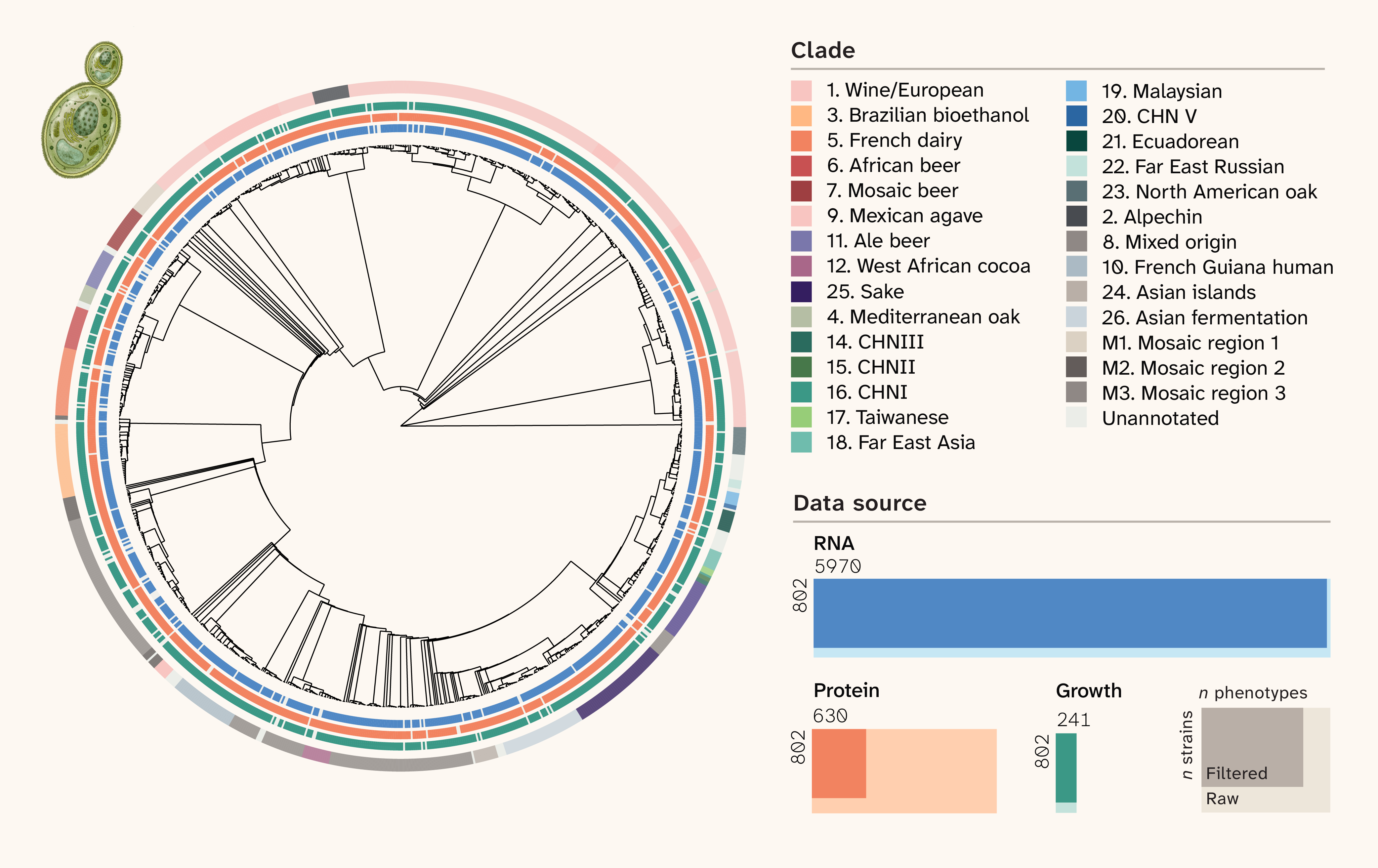
Figure 1. The structure of the dataset.
Neighbor-joining phylogeny of the 1,011 S. cerevisiae strains in the dataset. Clades are color-coded and correspond to the outermost bar. The other bars indicate the availability of measurements for the three phenotypic layers, which, moving from outside to inside, are growth (green), protein (orange), and RNA (blue). The rectangles indicate the raw and filtered dataset sizes for the three phenotypic layers. Filtered dataset sizes are indicated for each. Columns correspond to measurement number, and rows correspond to strain number (n = 802 for each).
Phenotypes are strongly compressed but not hierarchically ordered
We first asked how many effective dimensions organize variation within each phenotype layer. The number of measured traits defines the ambient dimensionality, but correlated traits can concentrate variation onto far fewer axes. Therefore, comparing effective dimension across RNA, protein abundance, and growth provides an initial test of whether phenotypic organization follows the expansion or funnel model.
We began with the participation ratio (PR), a global, linear summary of how evenly variance is distributed across the principal component axes (Figure 2, A). PR is high when many axes contribute comparably and low when a few axes dominate. We calculated it from the first 100 nonzero components, or all available components when fewer were present, and complemented it with two neighborhood-based estimates of intrinsic dimension. This allowed us to compare the dominant organization of variation across layers using both global and local summaries.
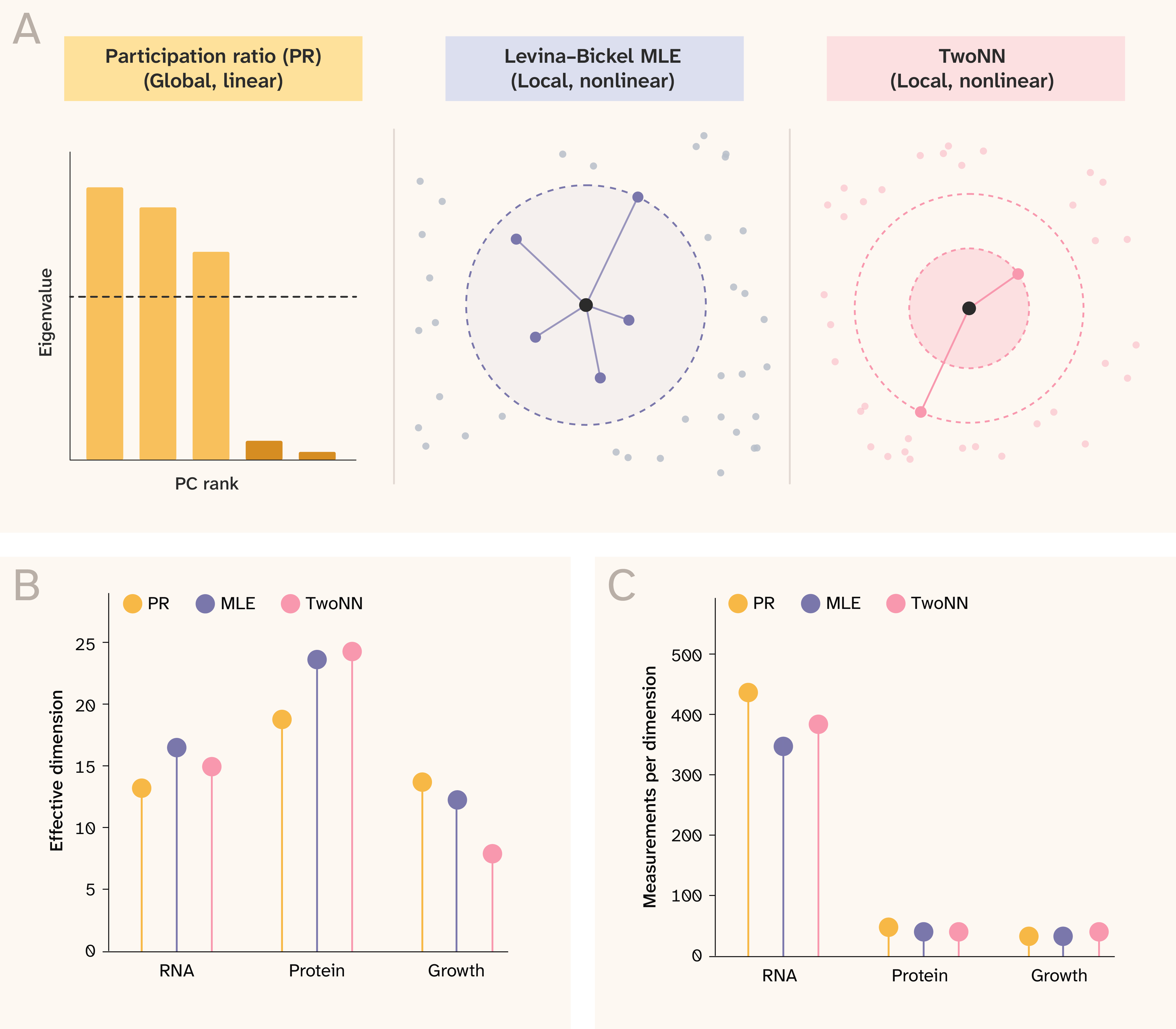
Figure 2. Phenotypic dimensionality is compressed but not hierarchical.
(A) Schematic of the three-dimensional estimators of dimensionality used. Participation ratio (PR) measures the fraction of principal component (PC) axes that are effectively occupied. Levina–Bickel maximum-likelihood estimation (MLE) and the two-nearest-neighbor (TwoNN) estimator estimate local dimensionality from nearest-neighbor distances. The dashed line in the PR estimation barplot marks the position of effective dimensions in the eigenvalue spectra.
(B) Effective dimensionality of RNA abundance, protein abundance, and growth phenotypes estimated by each method. Across all three estimators, phenotypic variation occupied only tens of effective dimensions despite hundreds to thousands of measured traits, and protein abundance had the highest dimensionality.
(C) Number of measured traits per effective dimension. Higher values indicate stronger compression relative to the number of measured traits. RNA abundance was the most compressed layer by this measure, whereas growth retained the most dimensional structure per measured phenotype.
The first result rejects the funnel model. PR didn't decrease from RNA to protein abundance to growth. RNA had the lowest PR (13.23), protein abundance the highest (18.76), and growth was intermediate (13.78) (Figure 2, B). Although each layer was strongly compressed relative to its ambient dimensionality, the degree of compression didn't track position in the molecular-to-organismal hierarchy — the proteome displayed most effective dimensions.
Because PR is derived from a global linear decomposition, it may misestimate dimensionality when phenotypic variation lies on curved or locally structured manifolds. We next asked whether the same pattern was recovered using two local, neighborhood-based estimators of intrinsic dimension: Levina-Bickel maximum-likelihood estimation (MLE) and TwoNN (Figure 2, B). Both methods supported the same qualitative conclusion. Levina–Bickel MLE estimated dimensions of 16.48, 23.61, and 12.24 for RNA, protein abundance, and growth, respectively, while TwoNN estimated 14.93, 24.26, and 7.88. In both cases, protein abundance again had the highest estimated dimensionality. Thus, across linear and nonlinear estimators, phenotypic variation occupied only tens of effective dimensions despite hundreds to thousands of measured traits, and dimensionality didn't decrease predictably across biological levels. The consistently high dimensionality of protein abundance is the opposite of what buffering would produce: if post-transcriptional regulation mainly dampened transcript-level variation, protein space should be more compressed than transcript space. Instead, protein abundance displays seemingly private axes of variation — favoring the expansion model at the protein layer.
We next considered whether the measurement model may still have explanatory power. Compression might simply track the number of measurements, and the phenotypic layers differed substantially in this respect: there were 5,970 transcript measurements, 630 protein measurements, and 241 growth phenotypes. We normalized PR by the number of measured traits to account for this. This inverted the pattern expected from trait counts alone: growth occupied the largest fraction of its measured space (5.72%), followed by protein abundance (2.98%) and RNA (0.22%) (Figure 2, C). Equivalently, one effective PR dimension corresponded to approximately 451 transcript measurements, 34 protein measurements, or 17 growth phenotypes. Thus, although growth didn't have the highest absolute dimensionality, it retained the most effective dimensional structure per measured trait. Trait counts alone, then, don't explain the ordering of the layers — a strike against the measurement model.
The measurement model's second concern is sampling: the ratio of measurement (p) to strain number (n) varied inconsistently across the phenotypic layers (RNA: p > n; protein: n ≈ p; growth: p < n), and when data dimensions exceed sample size, estimates can become unstable, and accurate reconstruction of data manifolds can be difficult. To test for this, we used rank-limited parallel analysis to estimate the number of principal components distinguishable from sampling noise at each phenotype layer. At the full panel size, RNA contained 55 detectable components, compared to 30 for protein and 24 for growth (Figure 3, A). The number of detectable components continued to increase with sample size across all three layers, most strongly for RNA; from 700 to 802 strains, the number of detectable components increased by 2.67 for RNA, 1.33 for protein, and 0.67 for growth (mean increase) (Figure 3, A). By contrast, intrinsic dimensionality estimates changed little over the same interval and were more stable overall (Figure 3, B). This suggests that the dominant axes of phenotypic variation are close to resolved at the current sample size, whereas weaker but detectable axes, particularly in the transcriptome, likely remain undersampled. Given this relative stability, we can conclude that each phenotypic layer occupies only a small fraction of what's been measured among S. cerevisiae strains. The compression we observe is therefore not a small-sample artifact, further challenging the measurement model.
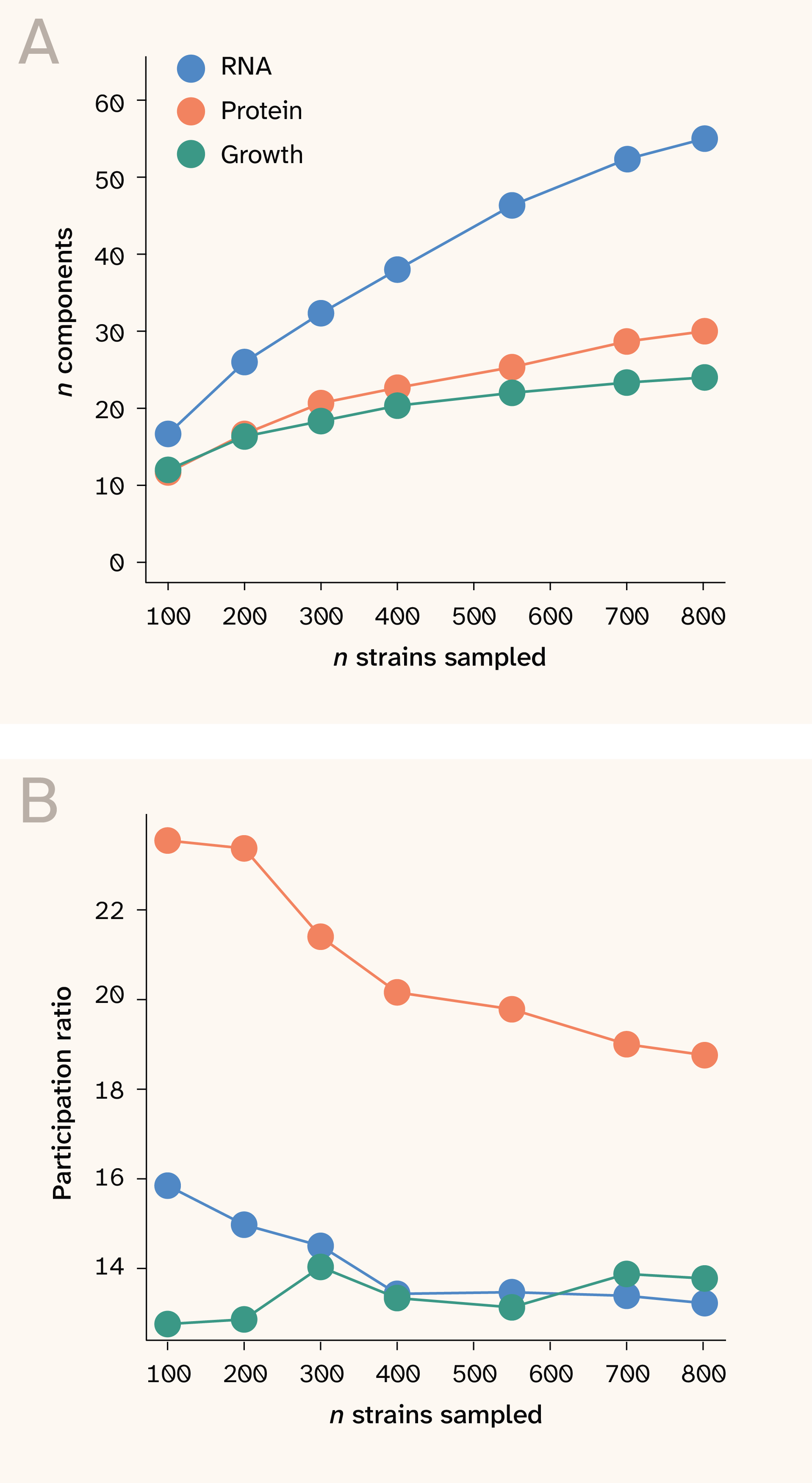
Figure 3. Dominant phenotypic dimensions are largely stable.
(A) Strain rarefaction of detectable principal components for each phenotypic layer. For each sample size, we subsampled strains and used rank-limited parallel analysis to infer the number of components with eigenvalues exceeding the permutation null.
(B) Strain rarefaction of PR. As in (A), PR was calculated by subsampling strains at each sample size.
These analyses show that yeast phenotypic variation is highly compressed: thousands of transcript, protein, and growth measurements resolve only on the order of tens of effective dimensions. In other words, this panel’s phenotypic diversity is generated by a few tens of coordinated programs rather than thousands of independently varying traits — and those programs aren't organized as a funnel. Variation isn't progressively integrated away as it approaches the organism; the proteome carries the most axes of all. But dimensionality describes only how many axes are needed to summarize variation, not how the occupied region is arranged. In what follows, we probe the spaces' geometries more deeply.
Phenotype spaces are continuous and geometrically structured
Small, local mutational steps traverse protein sequence space, but phenotype spaces need not work the same way — a space's shape determines how it can be traversed. For example, a low-dimensional phenotype space could reflect smooth gradients of variation, in which strains differ by degree along shared axes. Alternatively, it could reflect discrete phenotypic states, separated by gaps, thresholds, or constraints. These geometric differences reflect distinct evolutionary possibilities. A continuous space could imply that strains differ by degree along shared programs. In contrast, a partitioned space implies discrete phenotypic syndromes — distinct "kinds" of yeast, with gaps that lineages rarely cross. We therefore next asked whether yeast phenotype spaces are continuous or partitioned, how evenly strains occupy them, and whether their topology suggests simple clouds, loops, or branched connectivity.
We first used Hartigan dip tests to assess whether the leading axes of each phenotype space were multimodal, which could reflect the presence of discrete states or clusters. There was little evidence of multimodality (minimum p-values across five principal components (PCs): RNA = 0.949, protein = 0.412, growth = 0.785), suggesting that each space is continuous rather than discrete. Despite domestication, deep clade structure, and divergent ecologies, we detected no significant departures from unimodality along the tested axes.
The absence of detected multimodality, however, doesn't imply uniformity. We next assessed how unevenly strains occupied phenotypic space using Hopkins statistics, a complementary measure of spatial inhomogeneity. Hopkins statistics were higher than their matched Gaussian-null values in all three layers (RNA: 0.767 vs. 0.635; protein: 0.743 vs. 0.650; growth: 0.751 vs. 0.638), indicating nonuniform occupancy. A Gaussian cloud, like the null, has no clusters by construction, yet accounts for roughly half of the observed elevation. Given this large contribution, the remaining gap presumably reflects local clumping rather than discrete separation. Gaussian mixture models were consistent with this view: although the best fits selected multiple components (RNA: 8; protein: 7; growth: 9) (Figure 4), BIC improved slightly and then plateaued rather than peaking at a component count, the behavior expected of a mixture tiling a continuous density rather than recovering separated groups. Occupancy is therefore clumped rather than discrete: strains crowd into dense neighborhoods without forming distinct phenotypic clusters.
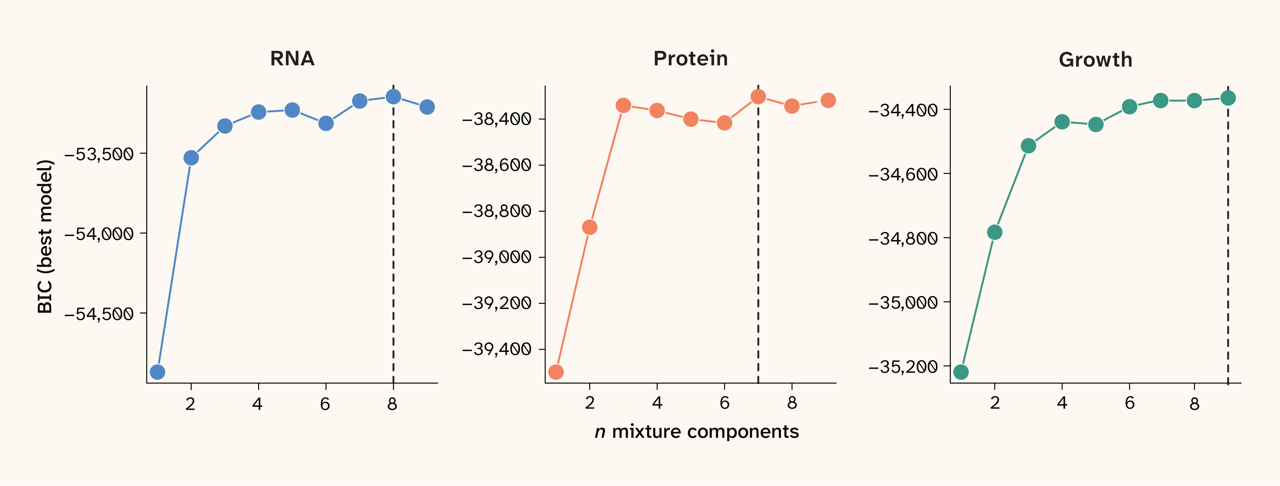
Figure 4. Phenotype spaces are continuous density gradients.
We fit Gaussian mixture models to the first eight principal component axes of each phenotype layer. Points correspond to the best Bayesian information criterion (BIC) for models with one to nine mixture components; dashed vertical lines indicate the model with the best BIC fit.
Continuous spaces of this type can arise from a variety of topologies. Each topology may lead to a different biological interpretation. For example, they may contain topological loops or “holes”: inaccessible regions in otherwise smooth spaces representing impossible trait combinations. Identifying features such as holes may aid in mapping the evolutionary accessibility of phenotypic space. One way to probe this is to measure persistent homology — the connectivity of space across distance scales (The approach).
Two features stood out when we looked at this. First, there was little evidence of persistent one-dimensional cycles (a signal of holes): excess persistence of the ten longest-lived loops was indistinguishable from matched flat nulls in every layer (z = 0.85, 1.55, and 0.12 for RNA, protein, and growth), and the data contained fewer and shorter-lived loops than a flat cloud of the same size and dimension (551 vs. 1,566 loops in RNA, z = −10.1) — the signature of clumping rather than of holes. Second, connected components persisted far longer than expected before merging. The longest-lived component survived to roughly twice the distance scale seen in flat nulls (RNA: 1.81 vs. 0.89, z = 29.9; protein: 1.48 vs. 0.89, z = 19.1; growth: 1.80 vs. 0.88, z = 28.2; 200 null draws per configuration), with the same pattern across the bulk of the distribution (95th percentile of component lifetimes, z = 20.6–25.6 across layers). The separation is complete: no null draw reached a component lifetime of 1.02, while the smallest observed value across layers was 1.48. Yeast phenotype spaces, therefore, are unevenly dense with persistent separation. Whether sparsely sampled regions connect denser groups remains unresolved. We next asked how distances and neighborhoods are organized within these spaces.
Beyond density and connectivity, phenotype spaces can differ in curvature — how neighborhoods of points spread or converge. In positive curvature, nearby paths tend to converge, as on the surface of a sphere; in flat spaces, distances behave approximately as in Euclidean space; and in negative curvature, paths tend to diverge, potentially producing tree-like patterns of separation (Figure 5, A). We measured curvature with two complementary metric diagnostics (The approach): Gromov delta, which asks how close sampled four-point configurations come to the additive relations that hold exactly in a tree, and the CAT criterion, which compares the distance from a third point to the midpoint of a pair against the value expected in a Euclidean comparison triangle. Both were calibrated on reference geometries of the same size and dimension. Gromov delta takes a value of 0 on a tree, 0.035 in hyperbolic space, 0.068 in flat space, and 0.092 on a sphere, while CAT takes −0.126, 0.021, and 0.194 in hyperbolic, flat, and spherical space, respectively. Because a history of lineage splitting should leave a negatively curved geometry behind, these diagnostics also test whether the bottlenecked continuum we observe reflects tree-like divergence.
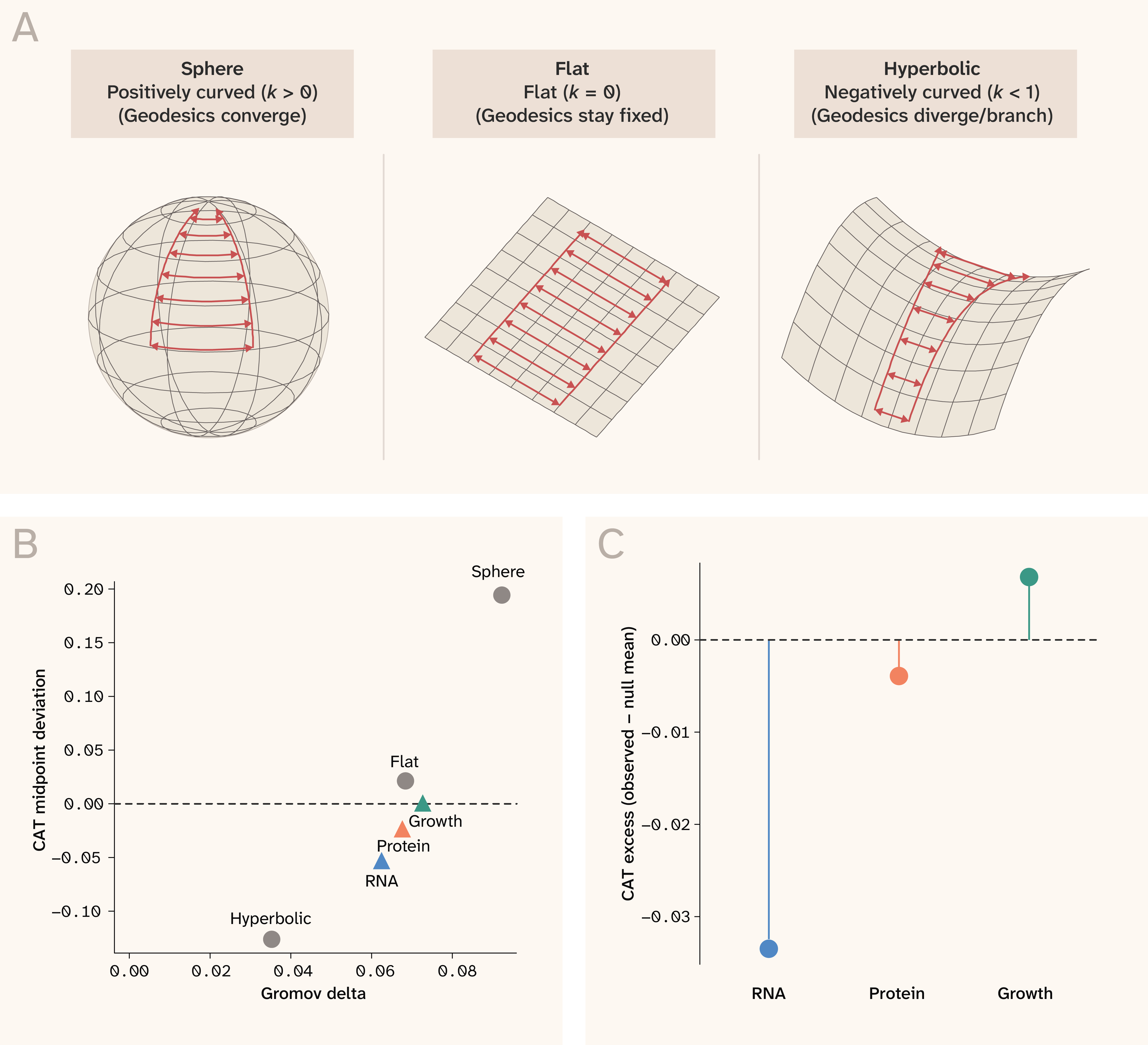
Figure 5. Assessing the geometry of phenotypic spaces.
(A) Schematic of the curvature regimes tested: positive curvature (sphere), where geodesics (red lines) converge; flat geometry, where geodesic spacing is consistent; and negative curvature (hyperbolic space), where geodesics diverge or branch.
(B) The relationship between Gromov delta and Cartan–Alexandrov–Toponogov (CAT) midpoint deviation for reference geometries (grey circles) and phenotype spaces (colored triangles). Gromov delta measures tree-likeness, with lower values indicating more negatively curved or branching structure. CAT midpoint deviation compares observed triangle structure with a flat Euclidean expectation, with negative values indicating thinner-than-flat triangles.
(C) CAT excess relative to nulls for each phenotype layer.
RNA showed the clearest evidence of negative curvature when compared to a flat null. Gromov delta was lower than expected under the null (0.0625 observed, excess = −0.0076, z = −4.78), and CAT shifted in the same direction, though less strongly (−0.054 observed, excess = −0.033, z = −1.73) (Figure 5, B–C). Against the calibration above, these values place RNA between the flat and hyperbolic references, but closer to the flat one. Protein abundance showed only a weak negative shift (delta excess = −0.0025, z = −1.55; CAT excess = −0.004, z = −0.20), and growth was indistinguishable from flat by both diagnostics (delta excess = 0.0011, z = 0.60; CAT excess = 0.007, z = 0.40). No layer showed evidence of positive curvature or a closed phenotype space.
Thus, all three spaces are continuous and locally uneven but display apparent differences in their curvature. RNA showed a modest shift toward a tree-like metric relative to its matched Gaussian null (CAT z = −1.73), but separate null comparisons do not establish curvature differences among layers or a monotonic trend across the biological hierarchy. Genetic ancestry is one possible contributor to this pattern, although a tree-like metric does not by itself identify clades or demonstrate sparse connections between them. We therefore next ask how much phenotypic variation is associated with ancestry and how that association differs across layers. These analyses characterize ancestry-associated variation; whether ancestry accounts for RNA’s modest curvature signature remains unresolved.
Ancestry shapes phenotype space but doesn't fully determine it
We first asked how much phenotypic variation could be explained by the known yeast clades (Figure 1). Across traits, clade identity explained a modest but consistent fraction of the variance, with mean trait-wise η2 values of 0.140 for RNA, 0.145 for protein, and 0.195 for growth (Figure 6, A). Thus, ancestry clearly contributes to the organization of phenotype space, but broad clade labels don't dominate the data: most phenotypic variance remains within lineages.
We next asked whether these ancestry-associated components of phenotype space had the same dimensional structure as the full phenotype space. They didn’t. Between-lineage variation was lower-dimensional than the total space, with participation ratios of 7.16 for RNA, 8.16 for protein, and 6.90 for growth (Figure 6, B). By contrast, clade-centered residual variation retained substantially more dimensional structure, with participation ratios of 12.73, 18.86, and 14.20 for RNA, protein, and growth, respectively. These residual values are close to the participation ratios of the full spaces (13.23, 18.76, and 13.78; Figure 2, B). This suggests that the dimensionality of yeast phenotype space is almost unchanged by ancestry. Between-lineage differences form a low-dimensional subspace embedded within a space whose geometry is otherwise intact. Clade differences contribute to phenotype-space geometry, but most effective dimensions aren't simply differences among major lineages.
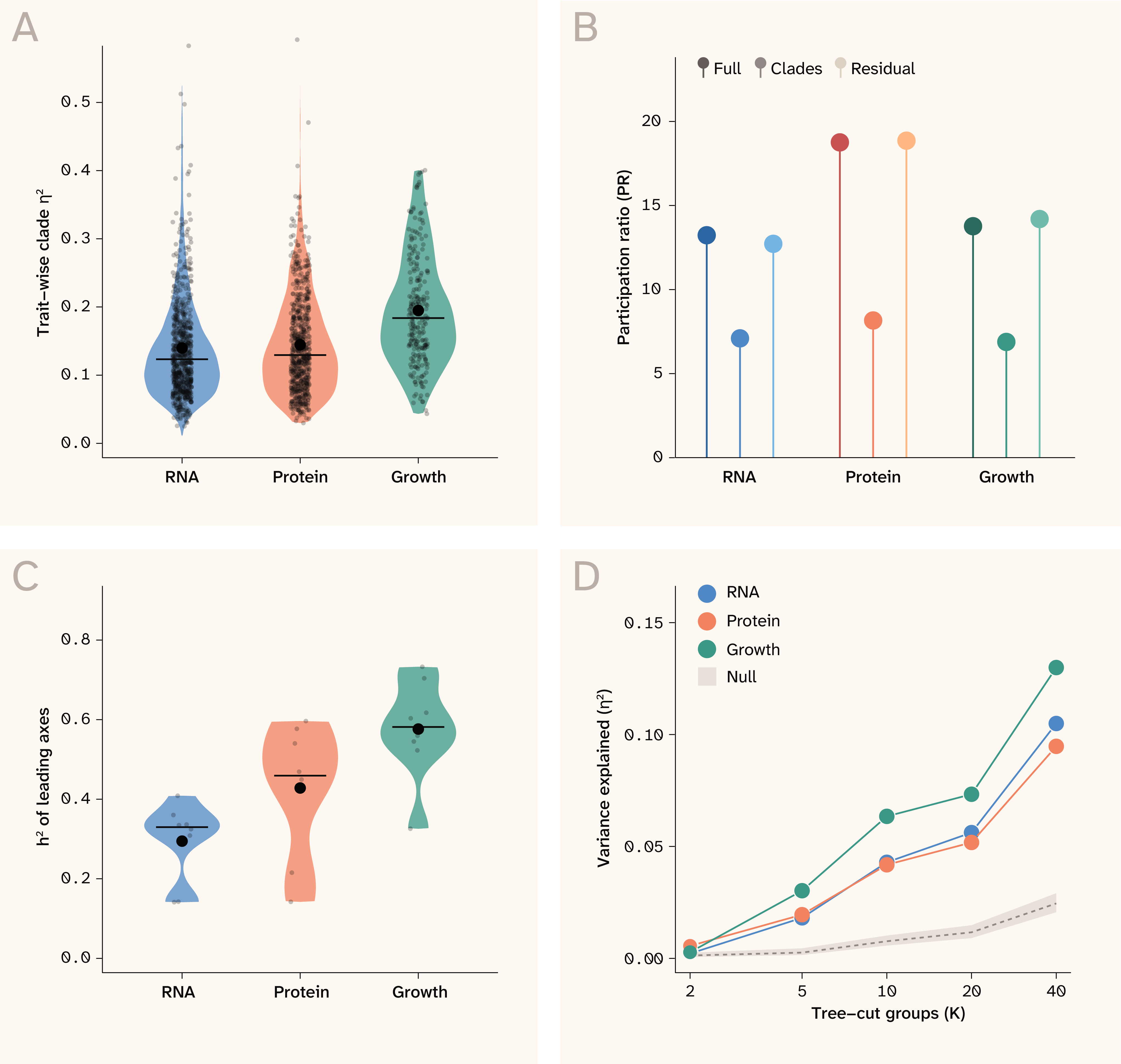
Figure 6. Ancestry shapes phenotype space but doesn't determine it.
(A) Distribution of trait-wise variance explained by major clade identity (η2) for RNA abundance, protein abundance, and growth. Points show individual traits, violins show the distribution across traits, and black marks indicate central tendency.
(B) PR of each full phenotype layer, the between-clade component, and the clade-centered residual component.
(C) Narrow-sense heritability (h2) of the leading phenotype axes for each layer, estimated from SNP-based relatedness.
(D) Mean variance explained by genotype-tree partitions of increasing granularity. Points and lines show observed η2 after cutting the SNP-distance tree into K groups; the gray band and dashed line show matched label-permutation nulls.
Genetic relatedness was associated with the dominant directions of phenotypic variation in all three layers. Variance-component models attributed, on average, 29.5% of leading-axis variation in RNA, 42.8% in protein, and 57.6% in growth to a relatedness kernel derived from SNP distances (Figure 6, C). These estimates characterize the leading axes of each full phenotype space. Although their interpretation depends on the relatedness kernel and assay reliability, they identify a consistent association between genetic and phenotypic structure across molecular and organismal measurements. This prompted us to ask at what depth of the genealogy phenotypic differentiation is most apparent.
Tree-cut analyses showed that the deepest genetic splits didn't drive phenotypic differentiation: K = 2 explained almost none of the variance (η2: RNA = 0.002, protein = 0.006, growth = 0.003), whereas finer partitions explained more (K = 40 η2: RNA = 0.105, protein = 0.095, growth = 0.130) (Figure 6, D). Because η2 increases mechanically with the number of groups, we compared each partition to permuted labels at matched K (The approach); the reported values exceed this null. Phenotypic differentiation, therefore, accumulates through fine-scale lineage structure rather than at the deepest divergences in the panel.
These genetic patterns run counter to the geometric ones. Narrow-sense heritability increased from RNA to protein to growth, while the curvature signature of tree-like divergence ran the other way, strongest in RNA and absent in growth. Genetic determination and lineage geometry are therefore partly dissociable: how reliably genotype predicts a phenotype isn't the same as how strongly the history of lineage splitting is imprinted on the shape of the space. This also helps explain why the funnel model failed. As variation propagates toward the organism, it becomes more genetically determined, not less, but also less tree-structured — a combination that simple propagation of transcript-level variation wouldn't produce.
Taken together, the single-layer analyses return a split verdict on the models we set out with. No single model describes yeast phenotype space. Dimensionality favors expansion: variation isn't integrated away as it approaches the organism. The proteome carries the most axes of any layer. Curvature, by contrast, follows the funnel: the tree-like structure in RNA fades to flat in growth. Heritability follows suit: genetic determination strengthens toward growth even as the influence of lineage history weakens. In all three layers, phenotypic variation is compressed to tens of axes, continuous rather than partitioned, clumped rather than uniform, heritable rather than noise, and shaped by lineage structure. Whether the layers share those axes — and what the unshared remainder implies about the current panel's coverage — is the question we finally turned to.
Heritable structure is asymmetric across layers
So far, each phenotypic layer has been characterized separately. This established how RNA, protein abundance, and growth spaces are structured on their own, but not how those spaces relate to one another. To do so, we explored whether shared axes of variation reveal how phenotypic structure is transformed across the biological hierarchy.
We first asked how much total variation in each layer could be recovered from the other measured layers. Cross-layer variance (see "The approach") was modest but highly structured, accounting for 12.1% of RNA variation, 13.8% of protein variation, and 13.7% of growth variation (Figure 7, A). RNA and protein showed similar partitions: protein uniquely explained 6.1% of RNA variation, RNA uniquely explained 6.2% of protein variation, and shared two-layer components accounted for an additional 5.0% and 6.4% of RNA and protein variation, respectively. Growth differed from the molecular layers. Nearly all cross-layer-explained growth variation was shared by RNA and protein together, rather than uniquely attributable to RNA alone (0.1%) or protein alone (2.7%). To place these values in context, we compared them with the reproducible variation remaining in each target layer. The measured cross-layer signal accounted for approximately 43% of the recoverable RNA and protein variation, but only 25% of the recoverable growth variation. Thus, the layers are neither independent nor redundant: RNA and protein recover a substantial fraction of one another’s reproducible structure, whereas growth contains much more heritable phenotypic structure that's not captured by the measured molecular layers.
These cross-layer associations show that each phenotypic layer contains measurable information about the others. Still, they don't by themselves indicate whether the shared signal is geometrically redundant or whether each layer contributes distinct axes of variation. We therefore asked whether combining RNA, protein, and growth phenotypes produced a joint phenotype space with fewer effective dimensions than expected if the layers captured independent strain structure. In the raw data, the combined participation ratio (PR) was 27.7 (Figure 7, B). To contextualize this value, we compared it with two reference distributions: a complete-overlap reference, in which the three layers were forced to share the same strain-level axes while retaining their layer-specific spectra, and an independence reference, in which the alignment among layers was broken by permuting strain identities across layers while preserving each layer’s internal geometry. The observed PR was far above the complete-overlap reference, which was centered near 15.6 (p < 0.01), but below the independence null, which was centered near 31.9 (p < 0.01). Thus, the joint phenotype space is significantly compressed relative to independent layers, but realizes only about a quarter of the compression expected if the layers were geometrically redundant. As above, this indicates that RNA, protein, and growth phenotypes share a measurable subset of axes, but that each layer also contributes substantial layer-specific structure to the overall phenotypic geometry.
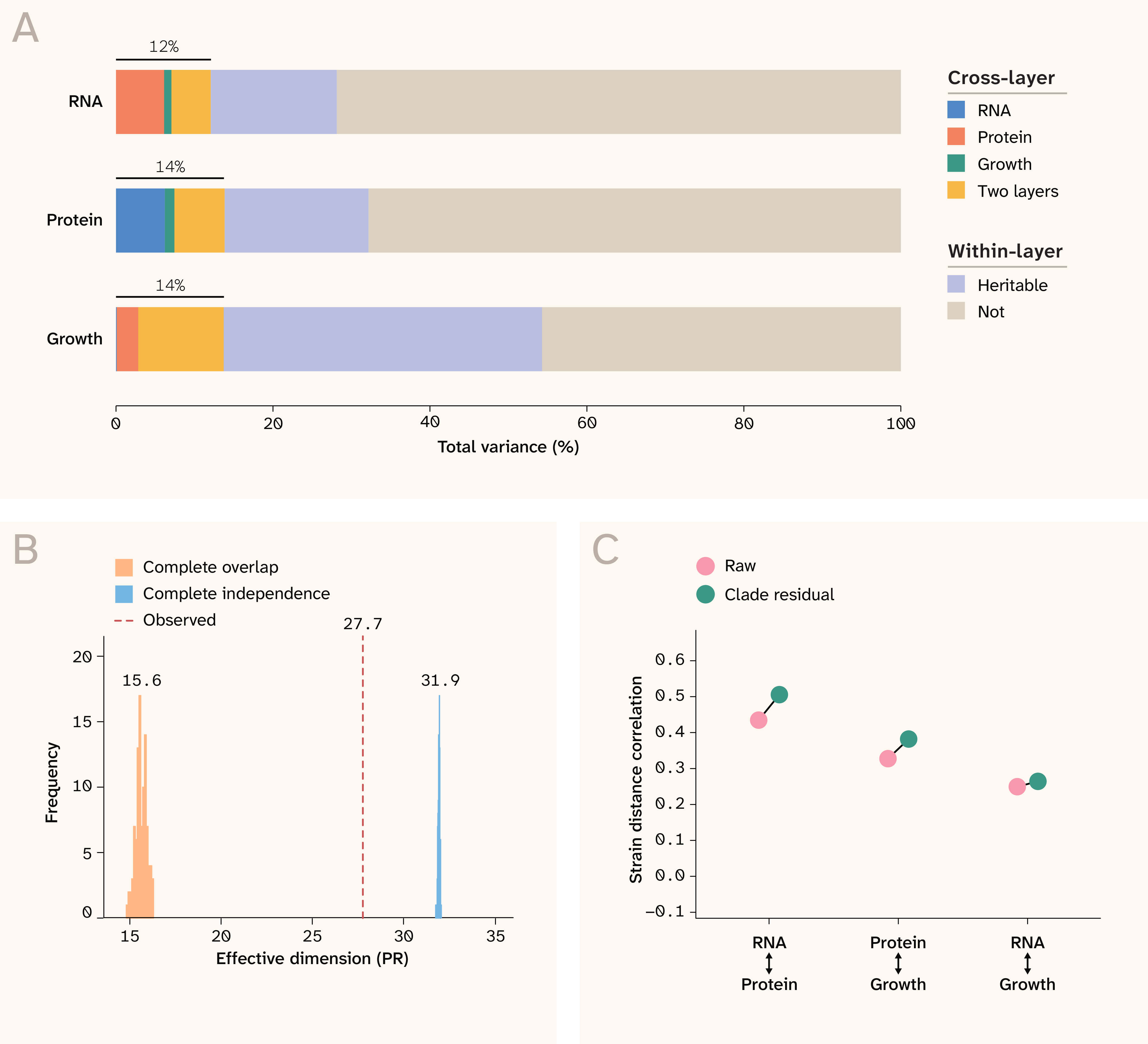
Figure 7. Cross-layer structure is incompletely recoverable.
(A) Cross-layer variance partitioning for each target phenotype layer. Colored segments show the fraction of total variance recovered from the other measured layers, partitioned into unique RNA, protein, growth, or shared two-layer components. The remaining variance is split into residual heritable variation and residual unexplained variation.
(B) Balanced joint participation ratio (PR) for the combined RNA, protein, and growth phenotype space. The observed joint PR is compared with a complete-overlap reference, in which layers share strain-level axes while retaining their spectra, and an independence reference, in which strain identities are permuted across layers while preserving each layer’s internal geometry.
(C) Pairwise strain-distance correlations between phenotype layers before and after removing major-clade effects.
Pairwise comparisons showed that this partial compression wasn't distributed uniformly across layers. RNA and protein occupied the most similar strain geometries, with a raw distance correlation of 0.435. In contrast, protein–growth and RNA–growth relationships were weaker but still structured, with distance correlations of 0.327 and 0.249, respectively. This ordering was largely preserved after removing major-clade effects, indicating that cross-layer alignment wasn't simply a consequence of broad population structure (RNA–protein: 0.506, protein–growth: 0.382, RNA–growth: 0.264; post-clade centering distance). In particular, RNA and protein remained strongly coupled in the clade-residual space, whereas growth exhibited a more distinct geometry. Thus, the shared component of the joint phenotype space appears strongest between molecular layers and progressively transforms at the level of growth.
These three views — cross-layer variance, joint dimensionality, and pairwise geometry — suggest an asymmetry. RNA and protein exhibit partially shared geometries and recover a substantial fraction of each other's reproducible structure. Growth is the most heritable layer (Figure 6, C), yet the measured molecular layers reconstruct only about a quarter of its recoverable variation. Almost none of it is attributable to either layer alone. Growth is, therefore, genetically anchored but molecularly under-determined by what’s been measured. Much of its estimated heritable variation remains unexplained by the tested linear predictors using RNA and protein measurements. Given what we can say from these data, information doesn't simply compress or expand across the hierarchy; it transforms, converging between the molecular layers and then diverging at the organism.
Implications
None of the three models we proposed explains the data on its own. Dimensionality is most consistent with expansion; curvature and heritability are more consistent with funneling; and normalizing by trait count reverses rather than eliminates the differences among layers. At least in this panel, the biological hierarchy isn't a pipe through which variation simply flows — expanding, compressing, or passing unchanged. Each layer reorganizes the variation present elsewhere in the system. Protein abundance contains axes not found in RNA. Growth shows a weaker tree-like metric signature than RNA, even as its leading axes become more heritable and its variation is more strongly associated with ancestry. What’s more, much of growth’s heritable variation can't be reconstructed from either molecular layer. The geometry of one layer, therefore, tells us surprisingly little about the geometry of the next. There's no reliable shortcut from a layer’s position in the biological hierarchy to the structure of its variation. The geometry within each phenotypic space, and the mappings between those spaces, are biological properties in their own right. They must be measured rather than assumed.
Lewontin’s genotype–phenotype (GP) map provides a useful way to interpret these results 56. He described evolution as a cycle of transformations: development maps genotypes and environments onto phenotypes, population processes filter which phenotypes persist, and inheritance and mutation shape the genotypes that follow. He argued that identifying the laws governing these transformations would bring us closer to a comprehensive theory of phenotypic evolution. Fifty years later, those laws remain elusive. Our results don't reveal those laws. Instead, they provide the types of patterns that candidate biological and measurement models should be tested against. Explaining the differences will require distinguishing how variation is organized in biology from how it's sampled and measured in each assay. Paired interventions and matched measurement contexts would help evaluate directional transformations that can't be inferred from this observational comparison alone.
Geometry also clarifies how much of the GP map the available data can resolve, and where additional sampling would pay off. The 6,841 traits analyzed here don't provide 6,841 independent views of the GP map. They collapse onto only a few dozen effective dimensions, and the transformations among them must be inferred from roughly 1,000 realized genotypes. The resource is wide but not deep: It measures many outcomes at relatively few positions in genotype and phenotype space. Rarefaction analyses mirror this. Our strain-rarefaction analyses suggest that sampling additional genotypes would reveal weaker dimensions of variation. Whether measuring additional traits would uncover new structure remains an open question. The incomplete alignment among layers points to a third source of information: phenotypic spaces not yet measured at all. The marginal value of a new measurement, therefore, depends less on how much data it adds than on which space it samples, and that value can be estimated in advance. Resolving the transformations among layers will require more paired measurements across molecular and organismal phenotypes, environments, time points, and controlled interventions — not simply more measurements in already saturated spaces.
Since this dataset is unusually well-suited to these questions, its limits are also instructive. Most current genotype–phenotype datasets are narrower on at least one axis. Human cohorts sample many genotypes, but molecular layers are typically measured in subsets of participants and in accessible tissues such as blood, rather than where organismal traits arise, and environments are uncontrolled 7, 57. Model-organism reference panels control the environment and allow replication, but they include tens to hundreds of genotypes rather than thousands 58–59. Single-cell perturbation atlases profile millions of cells, but usually in one molecular layer and a handful of genetic backgrounds 60–61. If a strain-matched panel of roughly 1,000 isolates is still wide but not deep, then most existing resources are likely under-resolved in ways their size obscures.
These limits also bear on models trained on such datasets. For example, many virtual-cell frameworks operationalize cellular state through RNA abundance and train models to reconstruct or predict transcriptomic profiles. Our results expose a limitation of treating that objective as a proxy for biological understanding. In this panel, growth is the most heritable layer but the least recoverable from RNA, and the correspondence between layers weakens toward the organismal phenotype. A model can therefore learn transcriptomic geometry accurately without learning the transformations that connect transcription to function. Transcriptomic fidelity isn't necessarily functional fidelity.
The 2025 Virtual Cell Challenge illustrates how difficult even the transcriptomic version of this problem remains. Models improved the discrimination of perturbations and the identification of differentially expressed genes, but didn't consistently outperform naive baselines across all evaluation criteria 62. The strongest entries also followed no single recipe: they included hybrids of pretrained neural networks and classical statistical methods, while a model operating on summary-level perturbation profiles placed among the top performers. This doesn’t mean that transcriptomic models are inherently uninformative. It does show that larger datasets and more expressive architectures don't, on their own, guarantee biological generalization. Together with the rarefaction patterns observed here, they suggest diminishing returns from scaling measurements within a single phenotypic space without also learning how that space relates to others.
These lessons extend beyond yeast and beyond virtual cells. Every phenotypic analysis, from comparative studies of morphology to association studies in human biobanks, rests on assumptions about the geometry of its data: how many independent axes it has, whether those axes are flat, and how samples relate to one another. Our results show that these properties vary across the layers of a single organism, so assumptions that hold for one type of measurement may fail for another. Methods that treat trait spaces as flat and low-dimensional will be closer to right for some layers than for others. Measuring geometry directly offers a way forward. It lets us test those assumptions rather than inherit them, compare datasets by what they can resolve rather than by their size, and study the transformations that generate phenotypes before the laws governing them are known.
Key takeaways
The organization — or “geometry” — of biological variation changes across different layers of life, so it should be measured rather than assumed.
- Thousands of measurements largely reflected a few dozen shared patterns, but those patterns differed across biological layers.
- Variation didn't consistently become simpler or more complex from RNA to proteins to growth. Each layer revealed a different picture.
- Growth differences were strongly associated with genetic differences, yet much of that variation remained unexplained by the measured RNA and protein levels. Accurately describing molecular activity, therefore, doesn't necessarily tell us how an organism will perform.
- Examining the organization, or “geometry,” of biological data can help researchers choose appropriate models and identify what to measure next.
Be the first to comment on this publication.