Purpose
Discrete information-theoretic measures summarize uncertainty and dependence without requiring a prespecified functional form, but their plugin estimators have null distributions that depend on sample size and contingency-table structure. This complicates inference across heterogeneous analyses and dataset and can make repeated permutation costly.
We present a likelihood-ratio framework for the discrete multinomial plugin setting. When the reported information quantity is the Kullback–Leibler divergence (KL) between the empirical distribution and the maximum-likelihood fit under a prespecified nested null, the exact identity converts information in bits to the likelihood-ratio deviance. Wilks' theorem then supplies an asymptotic chi-squared reference distribution, with degrees of freedom determined by the model comparison and prespecified support.
The framework applies directly to mutual information, conditional mutual information, fixed-reference KL goodness of fit, entropy deficit, and conditional entropy deficit. It yields distinct outputs for distinct purposes: a first-order-corrected information estimate in bits for effect magnitude, and a likelihood-ratio -value. It also gives the leading plugin correction a dual interpretation as estimator-bias correction and asymptotic null-mean centering.
We use simulations to evaluate mutual information (MI) and conditional mutual information (CMI) null moments, distributional calibration, sparse-table breakdown, and agreement with permutation across changes in sample size and conditioning cardinality. Sparse expected cell counts, rather than low degrees of freedom, were the principal finite-sample failure mode: The normal-equivalent representation handles small degrees of freedom, but it cannot repair a chi-squared approximation limited by sparsity. The particular count at which this transition appeared is specific to the simulation grids and is not proposed as a universal rule. The component identities and asymptotic results are classical; the contribution is their synthesis and operationalization for large, heterogeneous collections of discrete information-theoretic tests.
Introduction
Information-theoretic measures are attractive because they quantify uncertainty and statistical dependence without requiring a prespecified relationship between those variables (e.g., linear, additive, or monotone). For a discrete variable , entropy measures uncertainty about its state. Mutual information measures the reduction in uncertainty about one variable supplied by observing the other, and conditional mutual information measures the reduction in uncertainty provided by the set. Each of these can be formulated as a Kullback–Leibler () divergence, which quantifies the difference between two distributions. These are measures of information (conventionally bits when logarithms are base two) and are comparable 1–3.
One benefit of these values is the quantification of statistical dependence when the form of that dependence is unknown. In human genetics, for example, genotype–phenotype relationships may be additive, dominant, recessive, multiallelic, nonmonotone, or heterogeneous across sex, ancestry, or environment. A conventional single-variant genome-wide association test is highly efficient when its additive model is correct, but arbitrary categorical dependence requires additional model terms (often prohibitive at typical study scales) or an omnibus test 4–7. Mutual information (MI) and conditional mutual information (CMI) provide such omnibus summaries. They can therefore complement regression-based association analyses by testing for dependence without requiring the analyst to specify its form in advance.
A second application is repeated conditional-independence testing. Constraint-based causal-discovery, Bayesian-network learning, and ordered-trajectory methods repeatedly evaluate hypotheses of the form
while the size and state space of change across steps 8–11. CMI is a standard statistic for categorical conditional-independence testing 9–10. Local permutation-based testing (computationally expensive) or a fixed significance threshold across the changing state space (providing differing false positive rates across strata) are widely used 12.
In both cases, the practical obstacle to widespread use of information-theoretic measures isn’t their computation. It’s calculating well-calibrated (and thus comparable) significance for these estimates. In a genome-wide scan, loci can differ in sample size, number of genetic states at a given locus, missingness, and conditioning structure 4, 6–7. Each of these differences causes different significance thresholds for a locus–disease association. In causal discovery, the number of conditioning configurations can grow from one test to the next, again resulting in different significance thresholds as the trajectories progress. The paradigm presented here provides calibrated test and ranking statistics for any information-theoretic value that can be formulated as a Kullback–Leibler divergence (KL), including MI, CMI, entropy, and conditional entropy.
The problem
For discrete plugin estimators, the null mean and dispersion depend on both sample size and the dimensionality () of the relevant contingency-table model. The plugin MI of independent variables is upwardly biased; plugin entropy is negatively biased; and the null mean and variance of CMI grow as conditioning introduces additional strata. These effects, including mean corrections, are established in the finite-sample information-estimation literature 13–18. These biases have impacts on the utility of information-theoretic values. A fixed threshold on a raw information value can correspond to different false-positive probabilities in tables with different dimensions, and mean correction alone does not fix this problem.
Permutation, exact testing, and other resampling procedures provide general empirical calibration strategies, and they remain important when the estimator or sampling regime lies outside ordinary likelihood-ratio asymptotics 12, 19–20. Monte Carlo permutation -values also require careful finite-resolution calculation 21. These approaches are costly and can be prohibitive for large-scale data, such as current biobank datasets (often 500k samples and 1M parameters). Moreover, different information-theoretic measures are often presented with separate bias corrections, normalizations, or significance procedures, obscuring their shared statistical structure. The resulting methodological landscape can make information-theoretic inference appear more fragmented than it is.
Our approach: A synthesis of classical results
We therefore sought to establish an easily calculated, calibrated test statistic and evidence score that could be applied to MI, CMI, and other information theoretic values to enable genome-wide analyses with well-calibrated ranking statistics and significance thresholds.
The paper distinguishes between two inferential objects (Table 1).
| Quantity | Scientific role | Typical output |
|---|---|---|
| Information estimate | Magnitude of departure from a reference model | MI, CMI, entropy deficit, or KL divergence in bits |
| Calibrated evidence | Compatibility of the observed departure with a null model | Likelihood-ratio -value or normal-equivalent evidence () score |
Table 1. Information theoretic effect size vs. calibrated evidence.
A transformed evidence score is not an information-theoretic effect size. Conversely, an information estimate in bits does not by itself provide a significance threshold.
The mathematical ingredients needed to provide calibrated evidence for a statistical dependency in this case are classical. Shannon established entropy as a measure of uncertainty 1. Kullback and Leibler introduced relative information as a measure of statistical discrimination 2, and Kullback developed its role in hypothesis testing and contingency-table analysis 22. In the multinomial setting relevant here, the log-likelihood ratio between the empirical distribution and the maximum-likelihood distribution under a null model is exactly a sample-size-scaled KL divergence; this relationship is also standard in categorical-data treatments of likelihood-ratio testing 23–25. Independently, Wilks showed that likelihood-ratio statistics converge to chi-squared distributions under regularity conditions 26.
Connecting these two results provides the central inferential step:
where is the empirical distribution, is the maximum-likelihood distribution under the scientific null, and is the difference in model dimension. The equality is algebraic; the chi-squared distribution is asymptotic.
The contribution of the present work is the synthesis and its consequences. If an information statistic can be formulated as a KL divergence, the saturated-versus-null model pair and prespecified support determine the form and degrees of freedom of the test, the observed table determines , and Wilks calibration supplies the corresponding null moments, parametric -value, and common evidence (z-score) representation. MI, CMI, fixed-reference KL, maximum-entropy testing, and conditional maximum-entropy testing then become instances of one workflow rather than unrelated procedures. The section "Framework criterion" states the applicability criterion and clarifies why neighboring quantities (e.g., interaction information) require different inferential constructions.
The same synthesis clarifies classical first-order plugin corrections. Miller and Basharin developed leading entropy corrections, while later work treated transmitted information, conditional information, and the uncertainty of measured information quantities 13–14, 16–18. Under the chi-squared reference,
the corresponding fixed-support information statistic has a leading null expectation . Subtracting this expectation, the standard small sample bias correction mentioned above, is algebraically identical to centering on the mean of its asymptotic null. This doesn't replace the conventional interpretation as a first-order estimator-bias correction; it provides a second, likelihood-ratio interpretation of the same term.
Relation to prior work and scope
The likelihood-ratio interpretation of information statistics has a long history. McGill showed that sample-transmitted information could be used to measure and test association in multidimensional contingency tables 27. Kullback developed the representation of multinomial likelihood-ratio statistics as sample-size-scaled discrimination information 22, and the same connection underlies later information-theoretic treatments of contingency-table testing, partial association, and power 25, 28.
Finite-sample estimation of entropy and mutual information is, similarly, an established subject. Miller and Basharin derived leading entropy-bias terms 13–14; later work developed corrections and uncertainty calculations for transmitted information, conditional information, entropy, and MI 15–18. Roulston is especially close to the present standardization argument: He derived a transformation intended to map the MI of unrelated variables to a zero-mean, unit-variance normal test statistic as an analytic alternative to surrogate-data testing 29. Chance correction and standardization have also been developed for clustering-comparison null models 30–31.
For conditional independence in categorical data, the conditional or stratified likelihood-ratio test is also known. It appears in log-linear analyses of partial association 28, in information-theoretic Bayesian-network learning 9, and in modern work that explicitly treats the usual asymptotic CMI test as a standard baseline whose power deteriorates with increasing conditioning dimension 10. Exact and resampling-based alternatives remain important in finite, sparse, dependent, continuous, or mixed-data settings 12, 19–20. Recently, Goehle 32 obtained generalized chi-squared approximations for measured KL divergences between random exponential-family distributions using information geometry and a Bayesian central-limit argument; that setting is adjacent to, but distinct from, the saturated-versus-null multinomial likelihood ratios considered here.
Accordingly, the contribution of this paper is a synthesis and operational framework rather than a new likelihood-ratio identity or limiting theorem. The paper places the following elements in one explicit workflow: the null-model KL representation; Wilks calibration; null moments in information units; the dual interpretation of leading bias correction as asymptotic null-mean centering; support-aware degrees of freedom for conditional tables; and normal-equivalent representation of the resulting likelihood-ratio evidence. It applies that workflow consistently to MI, CMI, fixed-reference KL goodness of fit, entropy deficit, and conditional entropy deficit, and evaluates its finite-sample behavior in the large heterogeneous discrete-table regime motivated by the intended applications.
The framework applies only when the reported information quantity can be formulated as a KL divergence. It does not imply that every divergence or every information-theoretic functional is itself a likelihood-ratio statistic. For example, interaction information is a signed difference of MI and CMI rather than a KL divergence to one null-constrained model; inference requires a joint sampling distribution or an explicitly nested model comparison and is outside the present scope. Continuous estimators, data-adaptive discretization, boundary cases, and growing-dimensional tables likewise require estimator- or regime-specific treatment.
Contributions and organization
The paper makes five contributions:
- It applies the framework consistently to MI, CMI, entropy deficit, conditional entropy deficit, and fixed-reference KL goodness of fit.
- It shows that classical first-order bias corrections for information-theoretic values are algebraically the information-scaled versions of asymptotic chi-squared null-mean centering.
- It separates effect magnitude in bits from statistical evidence represented by , a -value, or a normal-equivalent score.
- It states an operational applicability criterion (see "Framework criterion"): An information quantity admits the direct construction when it is the KL divergence between the empirical distribution and the maximum-likelihood distribution under a prespecified nested multinomial null fitted to the same observations. The criterion delineates direct applicability and clarifies why signed composite statistics, the simple asymmetric KL divergence between separately estimated empirical distributions, nonmultinomial estimators, and nonregular or data-adaptive regimes require different inferential constructions.
- It evaluates finite-sample calibration across changes in sample size and conditioning cardinality and localizes the failure mode: Sparsity of expected cell counts, rather than low degrees of freedom, drives the observed breakdown. This distinction follows the structure of the construction, since the probability-integral transform addresses chi-squared skewness at any degrees of freedom but inherits whatever error is already present in the chi-squared approximation to . The analytic and permutation comparisons agree at the resolution available. The particular count at which the transition appeared is specific to these grids and is reported as a warning region, not a decision boundary.
The next section states the framework in its general multinomial form. Subsequent sections treat MI, CMI, entropy, conditional entropy, and fixed-reference KL as worked examples before evaluating the framework numerically.
The Kullback–Wilks framework
The framework requires only two steps. Kullback’s information-theoretic representation converts the relevant plugin statistic into a multinomial likelihood-ratio deviance, and Wilks' theorem supplies its asymptotic null distribution 22, 26. The remaining quantities — null moments, first-order correction, -value, and optional standardized evidence coordinates — follow directly.
Information divergence as a multinomial likelihood ratio
Consider independent observations allocated among cells. Let
be the saturated multinomial maximum-likelihood estimate, and let be the maximum-likelihood cell probability under a null model . The null model may be fixed, as in a goodness-of-fit test against a prespecified distribution, or it may be fitted subject to constraints, as in independence or conditional independence. This saturated-versus-null likelihood-ratio construction is standard in multinomial and categorical-data analysis 22–25.
Proposition 1 (Kullback representation). For the saturated multinomial alternative and a null-constrained maximum-likelihood distribution ,
when the divergence uses natural logarithms. In bits,
Proof. For the multinomial log likelihood, terms independent of the model probabilities cancel:
Changing from natural to base-two logarithms introduces the factor .
The equation above is exact for every observed table. It should not be read as saying that an arbitrary KL divergence between two estimated distributions is automatically a likelihood-ratio statistic. The reference distribution must be the distribution implied by the null likelihood for the same observations, and the alternative considered here is the empirical multinomial model 22, 25.
Wilks calibration
Proposition 2 (Wilks calibration). Suppose the null model is correctly specified and nested within the saturated multinomial model, with fixed dimension, identifiable parameters, and true probabilities in the interior of the parameter space. Then under ,
where is the saturated alternative 23, 26.
The conditions are worth separating because they delimit the ordinary Wilks regime. The numerical study in the section "The CDF representation is normal when the chi-squared input is adequate" examines primarily the expected-cell-count condition rather than attempting to characterize every possible failure mode:
- Fixed model dimension. The number of cells, and hence and , are held fixed as . State spaces that grow with the sample fall outside fixed-dimensional theory.pro
- Identifiable nested models. is nested within the saturated model, and both are identifiable.
- Interior parameters. The true probabilities lie in the interior of the parameter space. Structural zeros and boundary cases violate this and require non-standard limiting theory 33.
- Adequate expected cell counts. The chi-squared approximation requires cells to be sufficiently populated for the multinomial normal limit to hold. This is the condition we varried most directly in the numerical study; in the grids we examined, sparse expected counts produced the first visible deterioration in calibration 23, 34–36.
- Prespecified partitions. Categories, bins, and conditioning strata are fixed in advance. Partitions selected from the same data introduce effective parameters that doesn't count, making the nominal test anticonservative.
All five conditions delimit the ordinary chi-squared reference distribution rather than the algebraic identity in Proposition 1. That identity remains exact for an observed table whenever the saturated and null likelihood fits are well defined.
Conditions 1-3 and 5 are required for Wilks’ theorem to apply, but condition 4 limits the accuracy of the application of this synthesis. In other contexts, there are corrections for this limitation. Here, we demonstrate that this boundary is empirically near 18–20 expected observations per cell.
The primary inferential output is the upper-tail probability
Each analysis uses its own , null model, and . Once this calibration is valid, the resulting -values have the usual common-null interpretation even when the underlying tables differ.
Null moments in information units
Let
be the information statistic in bits. Because a chi-squared random variable has mean and variance , Propositions 1 and 2 imply the asymptotic null moments
These expressions expose the dependence of raw plugin information on both sample size and model dimension. Increasing contracts the null in information units; increasing the number of free departures from the null shifts and broadens it. Related bias and uncertainty calculations for entropy, transmitted information, conditional information, and MI appear throughout the finite-sample information-estimation literature 13–14, 16–18.
First-order correction as asymptotic null centering
Corollary 1 (dual interpretation of the leading correction). For the fixed-support information functionals treated in the following sections, define the first-order plugin correction
then
Thus, the leading information-scale correction is algebraically identical to centering the likelihood-ratio deviance on the mean of its asymptotic chi-squared null.
The identity in the equation above is exact after the correction term is defined. The statement that equals the finite-sample expectation of isn't exact; it follows from the asymptotic reference distribution. Under the regular fixed-support expansions used for entropy, MI, and conditional information, the correction has two compatible interpretations 13–14, 16, 18:
- It removes the leading plugin-estimator bias
- Under the null, it subtracts the leading chi-squared mean in information units.
This framing does not recast the historical corrections as something other than bias corrections. It shows that the same term also has a likelihood-ratio interpretation.
Three representations: Information, deviance, and standardized evidence
The framework yields related quantities with distinct roles.
Information effect. or its first-order-corrected form remains in bits. It quantifies the magnitude of departure from the reference model. The correction can be negative near a true boundary of zero; a negative corrected estimate does not imply negative population KL divergence.
Likelihood-ratio deviance. is the canonical test statistic. It incorporates both effect magnitude and sample size and is the natural scale for nested-model comparisons and deviance decompositions.
Moment-standardized statistic. The affine transformation
has mean zero and variance one under the chi-squared reference. We retain the name dimensionality normalization (DN) for continuity with the numerical development of this work. DN removes the first two null-moment dependencies but retains chi-squared skewness
It should therefore not be treated as standard normal when is small.
Normal-equivalent evidence score. Let and denote the chi-squared and standard-normal cumulative distribution functions (CDFs). Define
Roulston previously proposed an analytic normal transformation of MI for significance testing 29. The present use of the chi-squared CDF differs principally in making the null-model and degrees-of-freedom dependence explicit and in applying the same evidence coordinate across the broader family of likelihood-ratio statistics treated here. If followed the continuous chi-squared reference exactly, the probability-integral transform would make exactly standard normal for every . For finite contingency tables, the reference is asymptotic and the observed statistic is discrete; consequently, is standard normal only to the extent that the chi-squared approximation is accurate. It's a monotone representation of the same evidence as and adds no inferential content.
Framework criterion
An information-theoretic quantity belongs to this framework when it is the KL divergence between the empirical distribution and the maximum-likelihood distribution under a multinomial null. Different quantities correspond to different null models (Table 2).
| Quantity | Null model | Scientific question |
|---|---|---|
| Mutual information | Is there marginal dependence? | |
| Conditional mutual information | Is there dependence within conditioning strata? | |
| Fixed-reference KL | Does the distribution differ from a specified reference? | |
| Entropy deficit | uniform on fixed support | Is uncertainty below its support-constrained maximum? |
| Conditional entropy deficit | uniform within each stratum | Is uncertainty below its conditional maximum? |
Table 2. Null models and relevant hypotheses for Information quantities
The criterion also separates the quantities above from neighboring ones. Four cases fall outside the direct construction, each for a distinct reason.
- Signed or composite statistics. Interaction information is , a difference of two statistics computed on the same observations. It isn't a single nonnegative KL divergence to one null-constrained model, and because the two estimates are correlated, its null variance isn't the sum of theirs. Calibrated inference requires their joint sampling distribution or an explicitly nested model comparison 27–28.
- Simple divergences between separately estimated empirical distributions. The asymmetric quantity is not itself the likelihood-ratio deviance for a two-sample homogeneity test. That test instead uses each sample’s divergence from a pooled null-constrained estimate.
- Nonmultinomial estimators. Continuous nearest-neighbor and related estimators don't have the exact multinomial likelihood-ratio representation used here and require estimator-specific null theory or resampling 12.
- Nonregular or data-adaptive regimes. Boundary parameters, rapidly growing state spaces, and categories or partitions selected using the same data may invalidate the ordinary Wilks reference even when a likelihood-ratio statistic can still be defined 33.
Mutual information as a test of independence
This section instantiates the framework for the null . The null-model specification and prespecified support determine the form and degrees of freedom of the test; the observed table determines its likelihood-ratio statistic. Let and have and states, respectively, and let denote the observed counts in a contingency table. Write and for the row and column totals, and let .
The plugin estimator in bits is
Its population target is the KL divergence between the joint distribution and the product of its marginals. The corresponding null is
Under this null, the maximum-likelihood expected count is
The information-based contingency-table test is classical and appears in early work on transmitted information, Kullback’s statistical formulation, later information identities for contingency tables, and standard categorical-data treatments 22–23, 25, 27.
Proposition 3 (mutual information and the test). For every observed contingency table,
The equality is an immediate instance of Proposition 1. It's exact at every sample size and for every true distribution. Correctness of the null reference distribution is asymptotic 22–23, 25.
For a full-support table, the saturated joint model has free parameters, whereas the independence model has free parameters. Therefore
and under the regularity conditions of Wilks' theorem,
The resulting inferential quantities are
The -value is the primary hypothesis-testing output. The normal-equivalent score is useful for ranking, visualization, or integration with analyses expressed on standard-normal evidence scales; it's a representation of the same calibrated tail probability 29.
Null moments and the first-order plugin correction
The equations above give
The leading correction for MI is therefore
This is the MI instance of Corollary 1. Leading MI and conditional-information corrections of this form are derived directly in the later information-estimation literature 15–18. Under fixed support and positive cell probabilities, it removes the leading plugin bias; it isn't generally an exactly unbiased finite-sample estimator.
The corresponding DN statistic is
This standardizes the first two reference moments, but not the full distribution. In particular, a independence test has one degree of freedom and therefore retains substantial chi-squared skewness after affine standardization.
Interpretation in large-scale association analysis
For a locus–phenotype table, is a first-order-corrected effect estimate in bits: It estimates how much knowing the locus reduces uncertainty about the phenotype, without assigning a direction or imposing an additive genotype model. The pair measures evidence against marginal independence. This separation is analogous in role to reporting a regression coefficient together with its test statistic, while recognizing that the information-theoretic effect and a regression coefficient answer different scientific questions 4–6.
Locus-specific changes in , missingness, or observed genotype support alter the information-scale null moments. They don't prevent common evidence thresholds, provided each table is calibrated with its own likelihood-ratio statistic and valid degrees of freedom. When categories are removed because they're unobserved, however, the analyst must distinguish prespecified structural absence from random sampling zeros; the latter can signal a boundary or sparse-table regime where Wilks' approximation is unreliable 23, 33.
Conditional mutual information as a stratified likelihood-ratio test
This section instantiates the framework for the null . The conditional-independence model and prespecified stratum-specific supports determine the form and degrees of freedom of the test; the observed stratified table determines its likelihood-ratio statistic. Let , , and be discrete variables. The plugin conditional mutual information in bits is
where is the plugin MI calculated within stratum and . Equivalently,
The scientific null is conditional independence,
CMI and its asymptotic reference distribution are standard tools for categorical conditional-independence testing and Bayesian-network learning 3, 8–10.
Proposition 4 (CMI as a stratified statistic). Let be the likelihood-ratio statistic for independence of and within stratum . Then
Proof. Applying Proposition 3 within each stratum gives
Summing across strata and using yields
This representation is the classical conditional or stratified test, closely related to likelihood-ratio tests of partial association in log-linear models 9–10, 23, 28. The role of the present framework is to connect its likelihood-ratio calibration explicitly to the plugin CMI estimator, its null moments, and its information-scale correction.
Degrees of freedom
Suppose first that every one of the strata contains the same and admissible states. The saturated joint model has
free parameters. Under conditional independence,
and the model dimension is
The difference is
Under and Wilks' conditions,
These parameter counts are standard consequences of the conditional-independence/log-linear model 23–24, 28.
When the admissible supports differ across prespecified strata, the appropriate count is
where denotes the strata included in the model. This formula shouldn't be applied mechanically after deleting random zero-count categories: Such deletions can make the model selection data-adaptive and conceal boundary behavior. In sparse genomic tables, the nominal degrees of freedom and the adequacy of Wilks' approximation must therefore be assessed together 23, 33.
Null moments and calibrated evidence
The asymptotic information-scale moments are
In the full-support balanced case, the null mean is times the MI null mean for the same , , and , and the null standard deviation is times larger. This is the table-dimensional inflation that makes raw MI and CMI unsuitable as common evidence measures.
The first-order-corrected CMI is
with the leading conditional-information correction supported directly by finite-sample information-estimation work 10, 16, 18. The inferential outputs are
Calibrated MI and CMI -values, or their normal-equivalent coordinates, can be compared as evidence against their respective null hypotheses even when and table dimensions differ. They shouldn't be interpreted as measurements of the same population quantity. MI tests marginal independence, whereas CMI tests conditional independence. In particular,
is not a calibrated test of effect modification, confounding, or interaction.
Relation to conditional analyses in genetics and causal discovery
In genetics, asks whether genotype contains disease information within levels of a conditioning variable , such as sex or a prespecified population label. It is an omnibus conditional-dependence test. It can be sensitive to additive, dominant, recessive, multiallelic, nonmonotone, or context-dependent patterns, but it pays the degrees-of-freedom cost associated with that flexibility 4–5. A fully categorical regression containing all genotype main effects and genotype-by-condition interactions tests a closely related alternative with the same parameter count under the corresponding saturated categorical parameterization 23. Thus, the advantage isn't a cost-free interaction test; it's a functional-form-agnostic representation of arbitrary discrete conditional dependence.
In constraint-based causal discovery, the same calibration permits a fixed significance level to be applied while the conditioning table changes. Procedures that already compute test-specific -values from valid null distributions are already calibrated in this sense. The framework is most relevant when raw CMI thresholds are used, when analytic calibration hasn't been made explicit, or when repeated permutation is computationally prohibitive 9–12, 20. Continuous nearest-neighbor CMI estimators remain outside the present theory 12.
Fixed-reference KL divergence and entropy-based tests
The previous sections use null-constrained distributions estimated from the observed marginals. A simpler instance of the framework compares the empirical distribution with a fixed reference model. Entropy and conditional entropy enter as special cases when that reference is uniform.
Fixed-reference KL goodness of fit
Let have prespecified states, empirical probabilities , and a fixed reference distribution with on the admissible support. The plugin divergence in bits is
The null is
By Proposition 1,
If is completely specified, the null has no fitted multinomial parameters and
If belongs to a regular -parameter family whose parameters are fitted from the same observations, then the usual goodness-of-fit count is
provided the fitted model is identifiable and regular. These are standard multinomial goodness-of-fit results 22–24, 37.
The framework does not identify an arbitrary divergence between two independently estimated empirical distributions with a likelihood-ratio statistic. A two-sample homogeneity test, for example, uses each sample’s divergence from a pooled null-constrained estimate rather than simply . Such tests can be handled by likelihood-ratio theory, but the asymmetric pairwise divergence is not itself the relevant deviance 23–24.
Entropy deficit as a maximum-entropy test
Let be uniform on the fixed support. Shannon entropy in bits is
The divergence from uniformity is
Define the entropy deficit
Then
under
This is the ordinary multinomial likelihood-ratio goodness-of-fit test for uniformity expressed as a parametric test of maximum entropy on a fixed discrete support 1, 23–24. It isn't a generic test of the composite hypothesis for an arbitrary nonmaximal value . Parametric inference comparing Shannon diversities and entropies has other established formulations 38; the specific result here is the maximum-entropy/uniformity case.
The null mean of the entropy deficit is
Subtracting this mean from the deficit is equivalent to adding it to the plugin entropy:
The equation above is the Miller–Madow first-order entropy correction; closely related entropy-bias expansions were derived by Basharin and treated more generally in later work 13–14, 18. The sign is opposite to that for MI because the likelihood-ratio statistic is the deficit , not entropy itself. This is the entropy analog of Corollary 1: The leading entropy correction and asymptotic null centering of the deficit are the same operation written on opposite sides of the identity in the equation above.
Conditional entropy deficit
Let define prespecified strata and let have admissible states in stratum . The plugin conditional entropy is
The maximum conditional entropy allowed by the prespecified stratum-specific supports is
The conditional entropy deficit is
where is uniform on the admissible support in stratum . Therefore,
Under the null that is uniform within every stratum,
When every stratum has the same states, this reduces to . The construction is a direct stratified multinomial goodness-of-fit test 3, 23, 28.
This test asks whether uncertainty is maximal within every conditioning stratum. It's distinct from asking whether conditioning changes entropy. The latter question is
and is tested by the MI likelihood-ratio statistic described in the section "Mutual information as a test of independence."
Below we provide a summary table of the principal uses of this synthesis and articulate the estimand and the appropriate representation, null hypothesis, and degrees of freedom (Table 3).
Summary of principal instances
| Quantity in bits | KL representation | Null hypothesis | Degrees of freedom |
|---|---|---|---|
| uniformity / maximum entropy | |||
| conditional uniformity |
Table 3. Principal information-theoretic instances of the likelihood-ratio framework.
Degrees of freedom assume fixed, fully represented supports unless a general sum is shown.
In every row,
and the asymptotic -value is read from the chi-squared distribution with the row-specific degrees of freedom.
Numerical validation
The numerical study evaluates the consequences of the Kullback–Wilks synthesis in the setting that motivated the framework: discrete MI and CMI calculated from contingency tables with varying sample sizes and conditioning dimensions. The simulations are not intended to re-establish the classical likelihood-ratio results. They ask whether the asymptotic reference is accurate over the examined finite-sample regimes, whether the predicted null moments match empirical behavior, and where sparse cells cause the calibration to fail.
The existing experiments focus on MI and CMI. Fixed-reference KL and entropy-deficit tests are direct multinomial goodness-of-fit cases, and we don't simulate them separately in the present draft. Their inclusion in the mathematical framework doesn't depend on the MI/CMI simulations.
Software and reproducibility
Code, including a Python library and a script for figure generation, is available in this GitHub repository (DOI: 10.5281/zenodo.22214680)
We wrote all simulations in Python using NumPy (v1.26.4), SciPy (v1.11.4), and Matplotlib (v3.10.9) 39–41. Random draws used NumPy’s default_rng with seed 42. We reused the same estimator and transformation functions across experiments; parameter sweeps and null generators varied by figure.
Estimators and statistics
For a table, plugin MI was calculated as
For a table, plugin CMI was calculated as the stratum-weighted sum
For each estimate, the simulations formed
For numerical stability, the CDF values were clipped to before applying . In the full-support CMI simulations,
The historical DN parameterization describes the information-scale variance as proportional to , where . Equating that representation with the equation above gives
For the table used throughout, .
Null data generation
For most experiments, we used a genotype–disease null. We generated a genotype as the sum of two Bernoulli allele draws, giving . We generated disease as Bernoulli, giving . We assigned a population label to each observation, one of strata. The baseline allele frequency was 0.30. A linear frequency gradient and optional Gaussian perturbation could be introduced across strata, but we set both to zero for the null figures, so genotype and disease were independent both marginally and within strata.
For matched comparisons across conditioning cardinalities, we generated a partition at the largest and coarsened to obtain the smaller values. Thus, the same observations underlay the paired values at different in a simulation replicate.
Two experiments used alternative null generators. The degrees-of-freedom experiment sampled cell counts from a uniform multinomial over the cells. The validity-regime experiment generated each variable as an independent, uniform categorical variable. For power comparisons on tables, we fixed the marginals, numerically computed the joint cell probability corresponding to a target nonzero MI using scipy.optimize.brentq, and sampled counts from the resulting multinomial.
Monte Carlo evaluation
At each parameter setting, we generated independent replicate tables (default 500), computed the relevant statistics, and compared their empirical distributions with the predicted references. Evaluation included:
- quantile–quantile plots against the scaled chi-squared null for raw MI/CMI and against for ;
- Kolmogorov–Smirnov comparisons with the stated reference distribution;
- empirical mean, variance, skewness, and kurtosis;
- three estimates of chi-squared degrees of freedom: , , and maximum-likelihood fitting of a chi-squared distribution; and
- comparison with a label-permutation test in selected alternatives.
Non-rejection by a KS test is treated as evidence of agreement at the resolution of the simulation, not proof that the finite-sample distribution equals its asymptotic reference. In particular, the available replicate counts can't directly validate genome-wide tail probabilities such as .
Monte Carlo permutation -values should use a finite-sample correction such as , where is the number of permuted statistics at least as large as the observed statistic and is the number of random permutations 21.
Experiments
Correction progression across conditioning sizes (Figure 1). At , , and 500 replicates, we compared the statistic at a baseline with the statistic at each larger under four representations: raw information, first-order plugin centering (Basharin), DN, and the chi-squared-CDF transform.
Scaled chi-squared null across and (Figure 2 and Figure 3). Using the genotype–disease null, we compared with . Figure 2 varies at . Figure 3 varies at . Each setting uses 500 replicates.
Variance constant and degrees of freedom (Figure 4). We compared the predicted with empirical estimates for a table across at . We split three hundred tables into ten groups for repeated variance estimates. In a separate uniform-multinomial experiment, we evaluated across at using 2,000 replicates.
Normal-equivalent calibration (Figure 5). We compared with across and using 1,000 replicates per setting.
Sparse-cell validity regime (Figure 6). We generated independent-uniform draws across and using 500 replicates. We recorded the KS statistic and average expected count per cell, .
Tail behavior (Figure 7). At , , and 10,000 replicates, we compared raw information, DN, and CDF-transformed values in the upper empirical tail.
Analytic vs. permutation inference (Figure 8). For tables with target MI in bits and , we used 100 replicate tables and 200 permutations per table to compare detection power and per-table -values.
Numerical results
Progressive removal of null dependence on table dimension
Raw plugin information changed systematically with conditioning cardinality in the matched-table comparison (Figure 1, A). Across the values we examined, the normalized mean RMSE was , and the normalized slope deviation was 1.0914. Subtracting the first-order plugin term removed most of the mean shift but left the changing dispersion intact (Figure 1, B; normalized mean RMSE , normalized slope deviation 1.0914). Dividing the centered statistic by the chi-squared null standard deviation aligned the first two moments (Figure 1, C; normalized mean RMSE , normalized slope deviation 0.0266), while the residual chi-squared skewness remained degree-of-freedom dependent. Mapping the full chi-squared reference through its CDF produced the closest agreement across conditioning sizes (Figure 1, D; normalized mean RMSE , normalized slope deviation 0.0393).
These panels illustrate the different roles of the operations. First-order plugin centering addresses the leading null location, DN aligns location and scale, and the CDF transform expresses each table’s chi-squared tail coordinate on the same standard-normal reference. Only the final step addresses the full reference shape. These operations have direct antecedents in the finite-sample information and analytic MI-significance literature 16–18, 29; the simulations here validate their implementation and operating regime in the present CMI setting rather than the classical identities themselves.
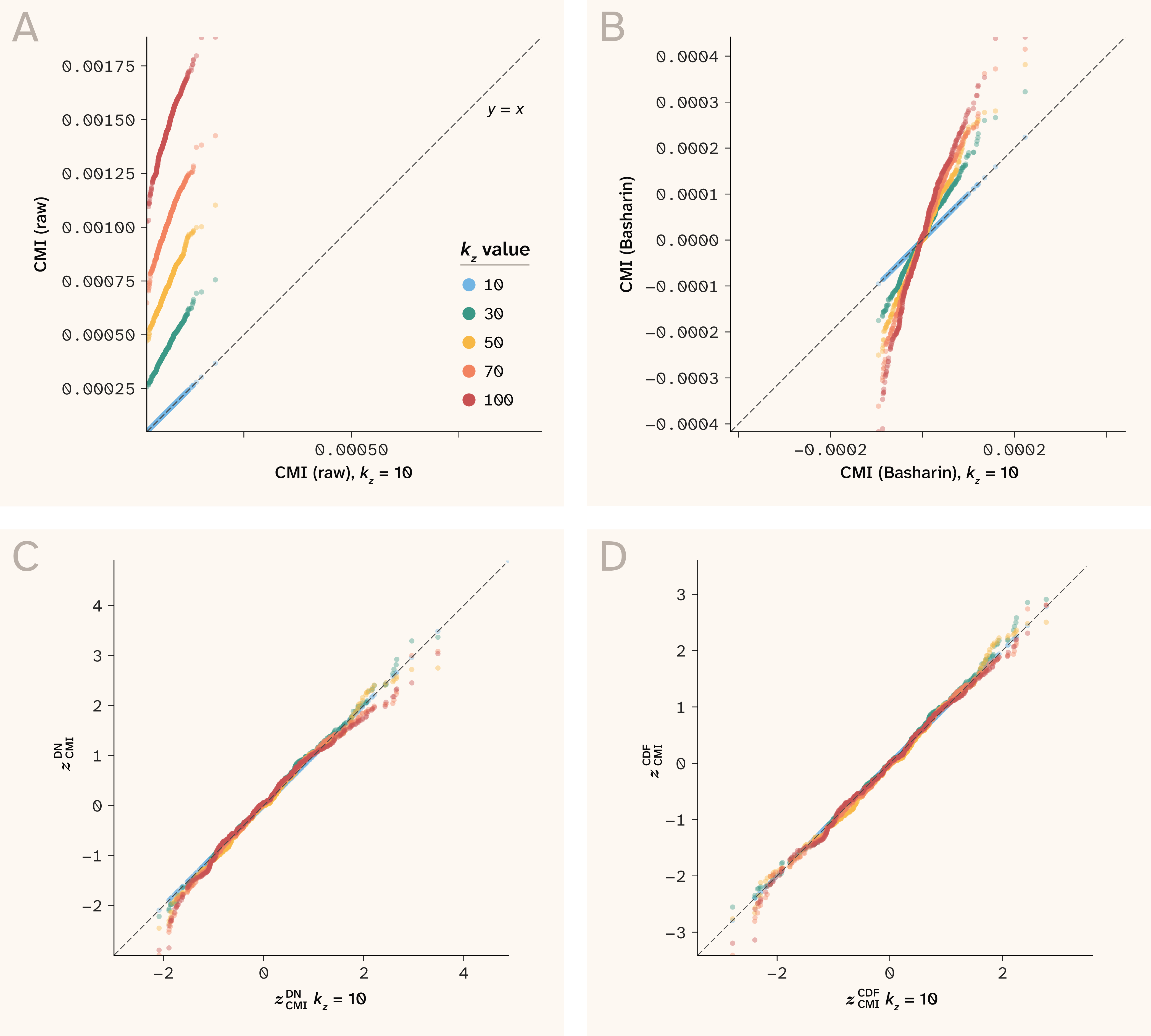
Figure 1. Progression from raw information to a common null-evidence coordinates across conditioning dimensions.
The panels compare CMI-null realizations as the number of conditioning strata changes.
(A) Raw plugin information.
(B) First-order plugin correction (labeled “Basharin”).
(C) First and second order correction (dimensionality normalization, ).
(D) Chi-squared-CDF normal-equivalent score, . Simulations used and tables with . The final panel should be interpreted as alignment of evidence under the respective nulls, not equality of CMI effect magnitudes across differing dimensions.
The scaled plugin statistic follows the predicted chi-squared null
Across changes in conditioning cardinality, the empirical plugin statistic agreed with the scaled chi-squared reference and with the directly calculated likelihood-ratio statistic (Figure 2). All reported KS comparisons in this dense-table experiment had . The same pattern held across changes in sample size at fixed (Figure 3). These results reproduce the expected consequence of the classical Kullback representation and Wilks calibration: The information estimate and are algebraically the same statistic in different units, while the quality of the chi-squared approximation depends on the sampling regime 22–23, 26.
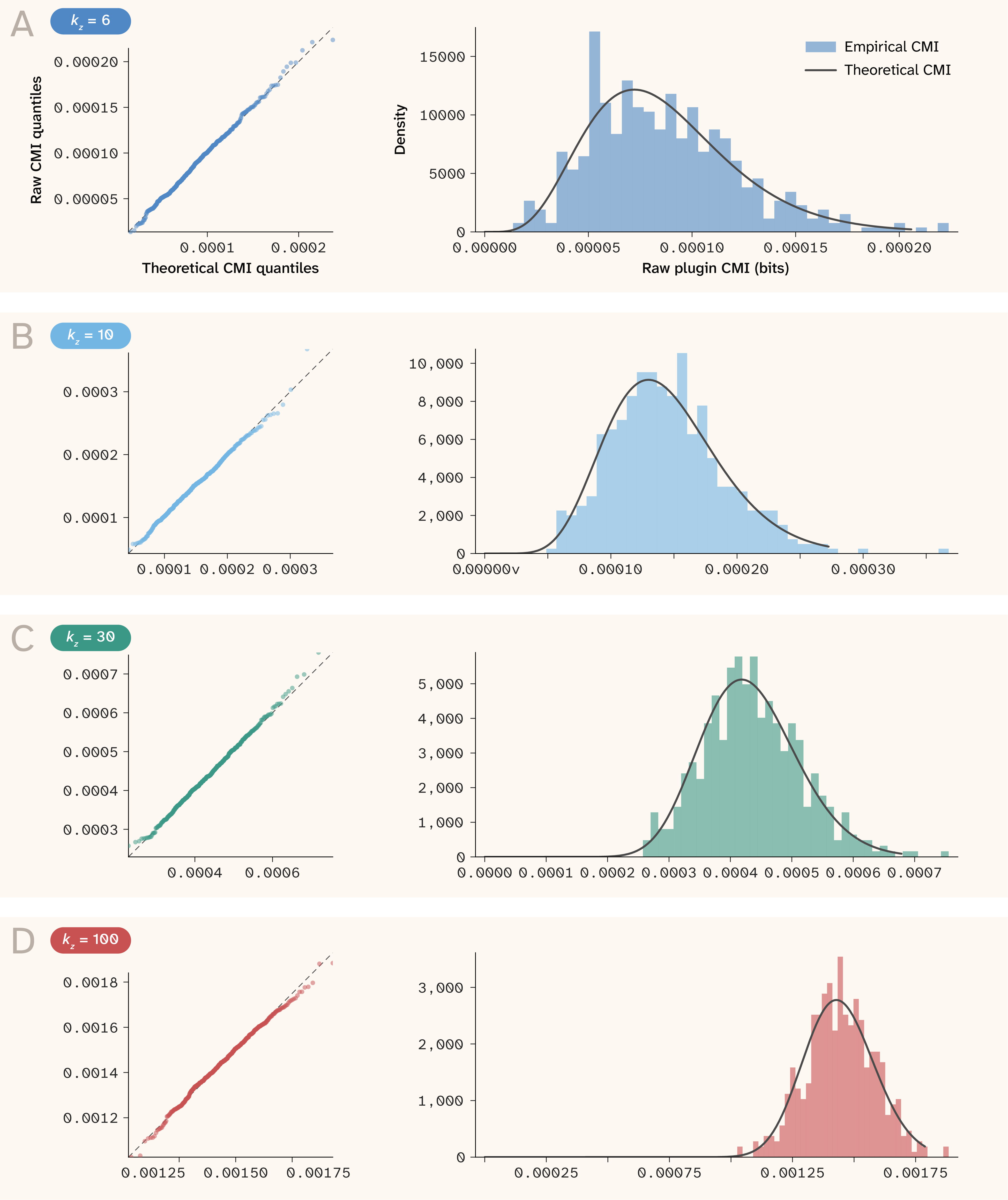
Figure 2. The plugin CMI statistic follows its scaled chi-squared reference across conditioning-table sizes.
At left, each row shows Empirical vs. theoretical quantiles. At right, each row shows Empirical densities and the corresponding scaled chi-squared densities. ; table size ; .
(A) = 6
(B) = 10
(C) = 30
(D) = 100
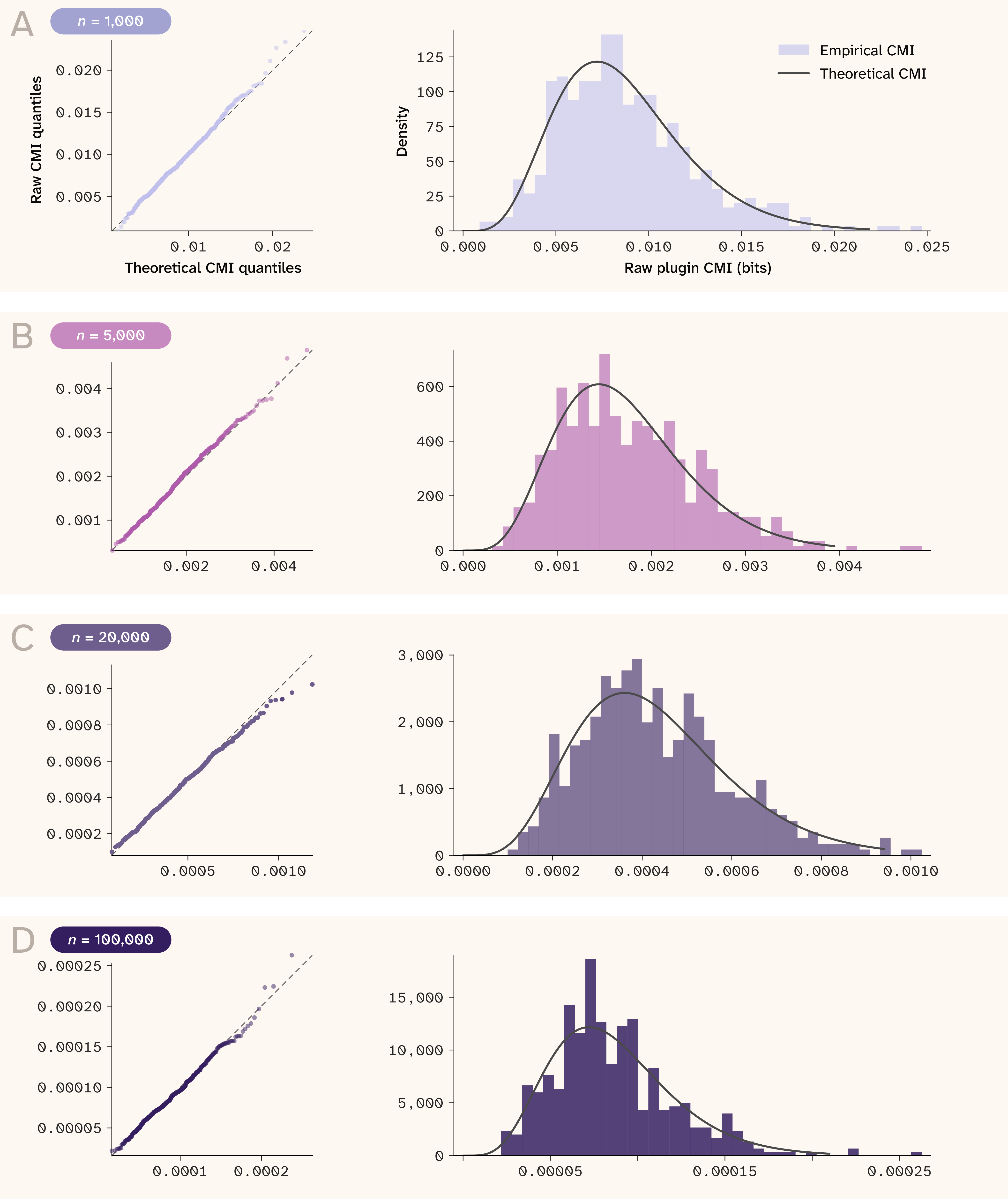
Figure 3. The plugin CMI statistic follows its scaled chi-squared reference across sample sizes.
At left, each row shows empirical vs. theoretical quantiles. At right, each row shows empirical densities and the corresponding scaled chi-squared densities.Table size ; .
(A) 1,000
(B) 5,000
(C) 20,000
(D) 100,000
Empirical variance and degrees of freedom match the framework
The empirical information-scale standard-deviation constant for the table was 0.588, compared with the theoretical value 0.589 from the equation above (Figure 4, A). Across conditioning cardinalities, degrees of freedom estimated from the mean, variance, and maximum-likelihood chi-squared fit closely tracked the theoretical value (Figure 4, B). The regression of empirical on theoretical degrees of freedom had slope 1.017 and correlation ; the reported regressions had .
This experiment is best viewed as a numerical check on the null-moment consequences of the framework rather than an independent derivation of the variance correction. Once the chi-squared reference is accepted, both the variance and the degree-of-freedom scaling follow analytically; related MI variance and error calculations have been derived by other routes 17–18.
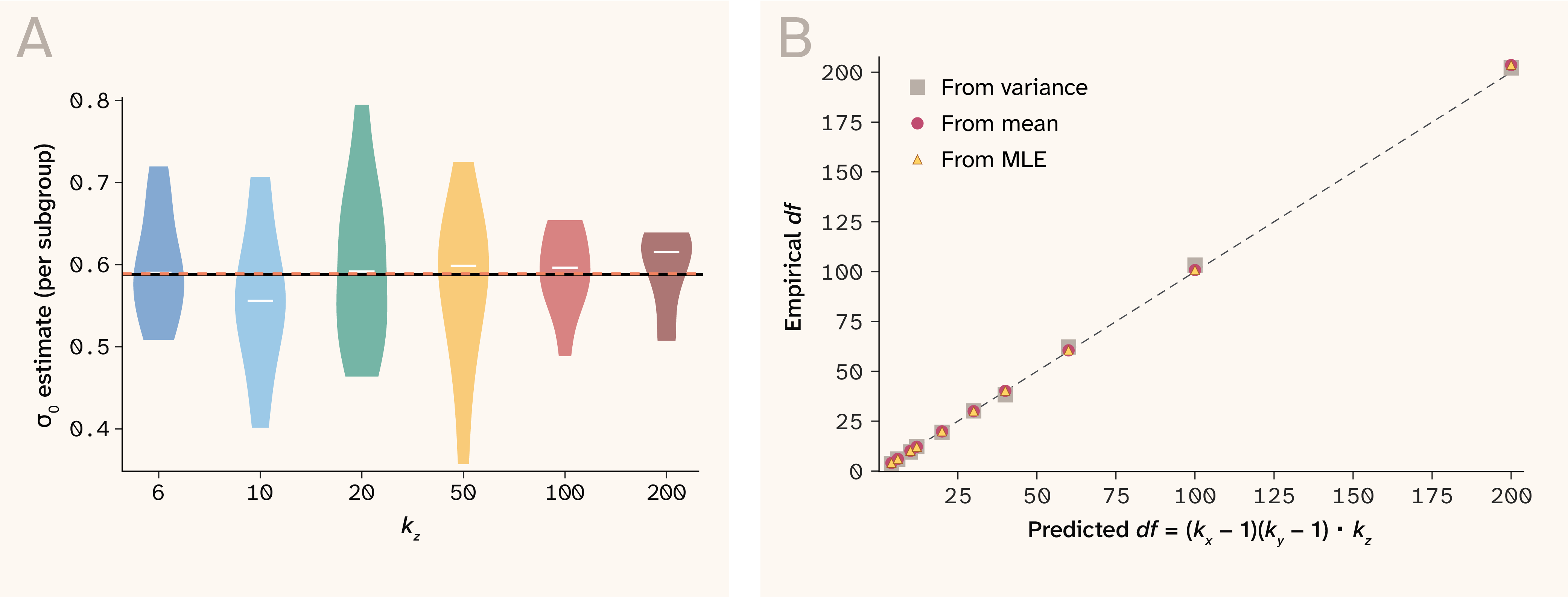
Figure 4. Empirical variance and degrees of freedom agree with the theoretical chi-squared moments.
(A) Repeated estimates of the information-scale standard-deviation constant across for tables at . The empirical mean (0.588, solid black line) and theoretical value (0.589, dashed salmon line) nearly coincide. Distributional medians indicated by white bars.
(B) Empirical degrees of freedom estimated from the mean, variance, and maximum-likelihood chi-squared fit vs. . MLE: Maximum likelihood estimation.
The CDF representation is normal when the chi-squared input is adequate
The normal-equivalent score was close to across most of the sample-size and table-dimension combinations examined (Figure 5). Sparse combinations departed from the reference, most clearly at and . This behavior is consistent with the framework: The CDF mapping handles chi-squared skewness at small or moderate degrees of freedom, but it can't correct a poor chi-squared approximation caused by sparse cells.
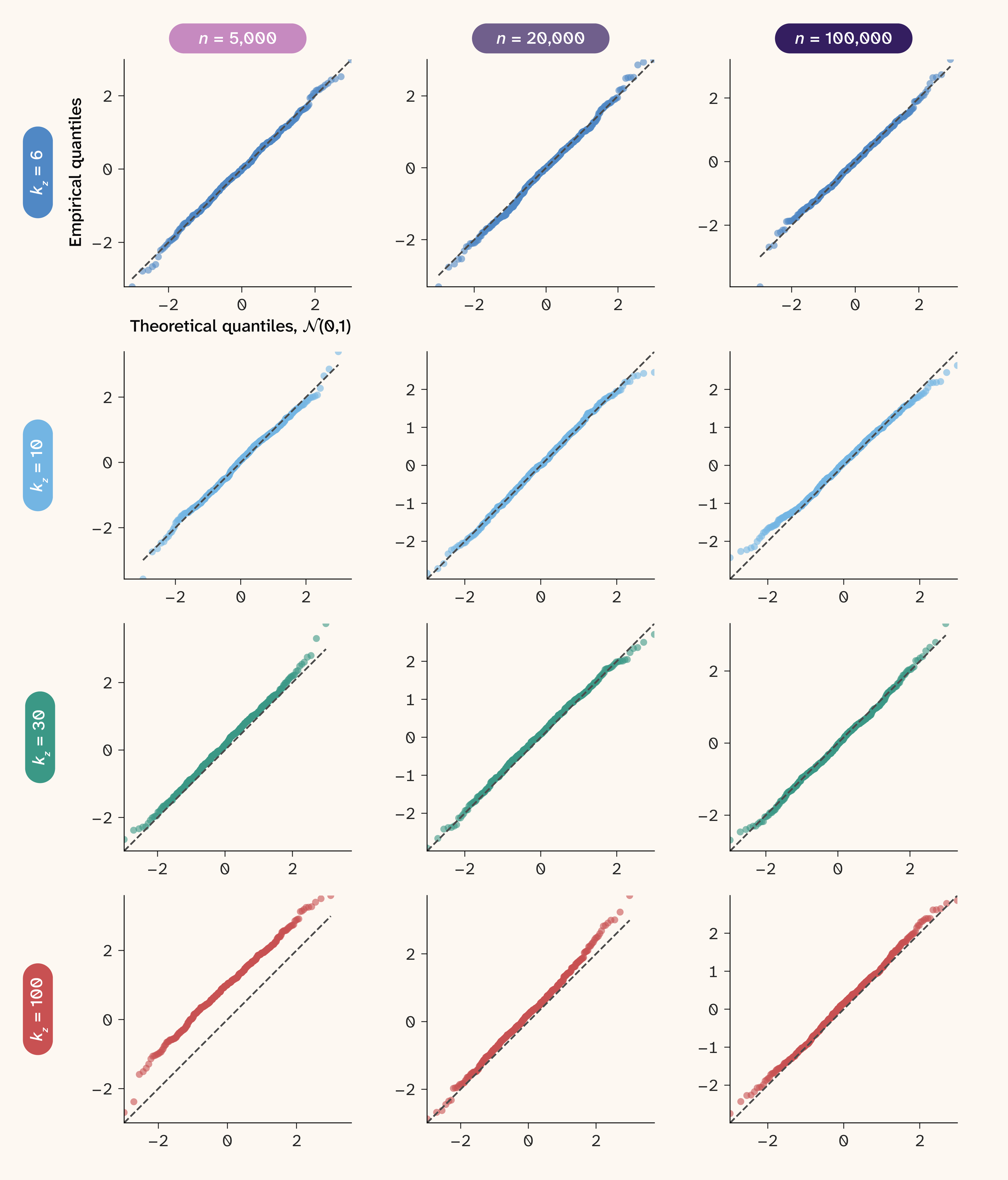
Figure 5. Normal-equivalent evidence scores across sample size and conditioning cardinality.
QQ plots compare empirical values with . Columns vary ; rows vary . Deviations concentrate in the sparsest combinations, where the chi-squared approximation to is least accurate.
In the balanced validity grid we examined here, departures from normal-equivalent calibration became common as average expected counts fell below approximately 18–20 per cell (Figure 6). This provides an empirical warning region for these table geometries, not a general operating boundary or a stand-alone rule for replacing permutation. The transition is specific to the null generators, table geometries, replicate counts, and KS diagnostic used here. Calibration can also depend on the minimum and distribution of expected counts, marginal imbalance, structural zeros, the target tail probability, and other departures from regular multinomial conditions, as established in the broader sparse-multinomial literature 23, 34–36.
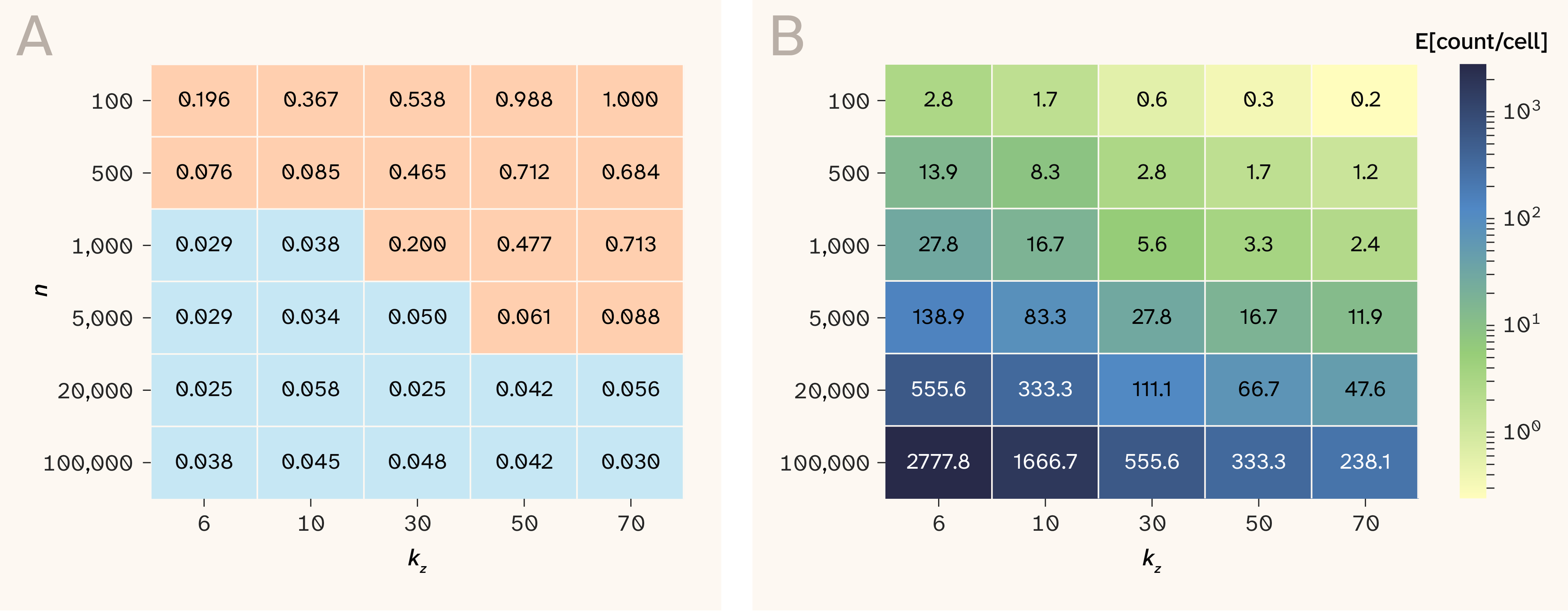
Figure 6. Sparse-cell boundaries for applicability of this paradigm.
(A) KS diagnostic for across and . Blue denotes and orange .
(B) Average expected count per table cell, . The transition near 20 counts per cell is specific to this grid and marks deterioration of the chi-squared input approximation, not failure of the probability-integral transform itself.
The upper-tail comparison likewise showed progressive improvement from raw information to DN and then to the CDF representation (Figure 7). DN retained degree-of-freedom-dependent chi-squared tails, whereas the CDF representation followed the normal reference closely in the dense regimes examined.
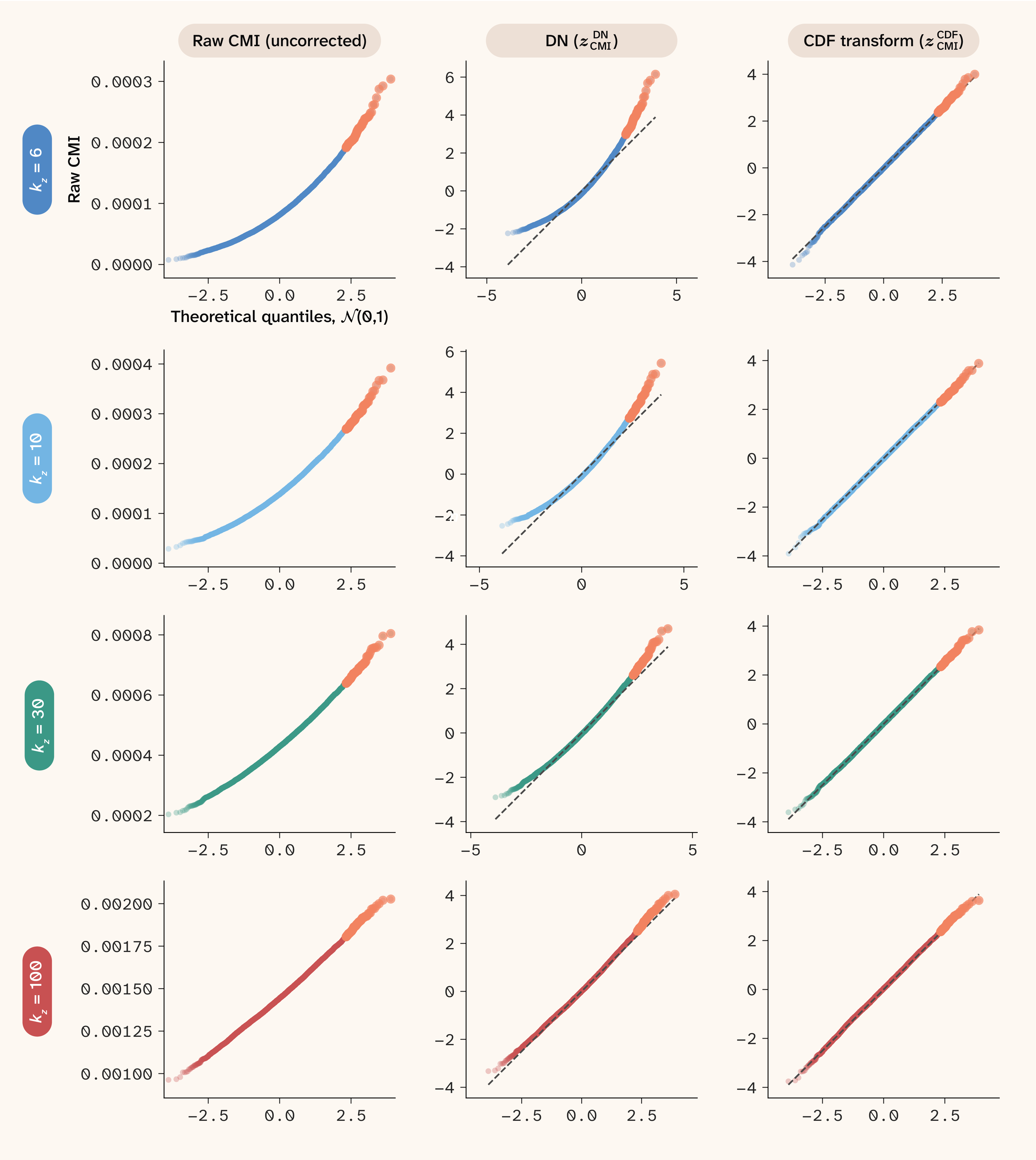
Figure 7. Upper-tail behavior of raw, moment-standardized, and cumulative distribution function (CDF)-transformed statistics.
Columns show raw information, DN, and ; rows vary conditioning cardinality. The CDF representation accounts for the full chi-squared reference shape, while DN retains residual skewness at lower degrees of freedom.
Analytic and permutation inference agree at the available resolution
Across the alternatives examined, analytic and permutation estimates of detection power were close (Figure 8, A). Per-table -values agreed where the 200-permutation procedure had sufficient resolution (Figure 8, B). The horizontal floor reflects the finite resolution of the chosen number of permutations; below that floor, the comparison cannot validate the analytic tail probability. Exact and permutation-based MI tests provide important alternatives in regimes where asymptotic calibration is unsuitable 19, 21.
The experiment supports analytic likelihood-ratio calibration as a computational alternative in well-populated discrete tables, but it does not establish equivalence in genome-wide extreme tails. More permutations, importance sampling, or substantially larger null simulations would be required for direct empirical assessment at such thresholds.
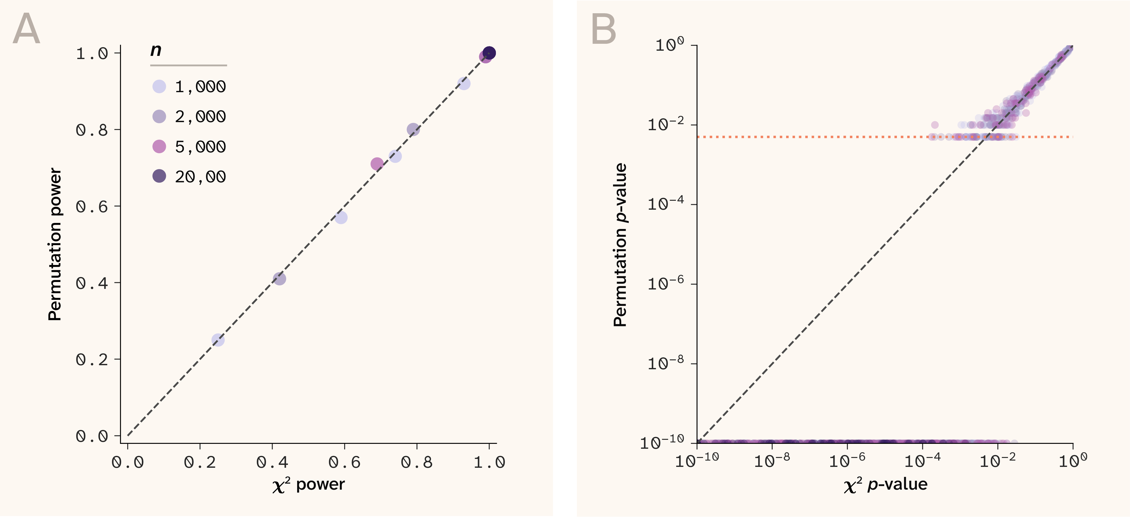
Figure 8. Analytic chi-squared and permutation inference in alternatives.
(A) Detection power from the permutation test vs. the analytic likelihood-ratio test across sample sizes and target MI values.
(B) Per-table permutation and analytic -values. The dotted horizontal line marks the permutation-resolution floor. Only panels A and B of the original figure are shown because they compare like inferential quantities.
Summary of the numerical evidence
Together, the simulations support four conclusions within the regimes we examined. First, the plugin MI and CMI statistics are numerically identical to the corresponding likelihood-ratio deviances after unit conversion. Second, their null means, variances, and degrees of freedom follow the chi-squared predictions in dense tables. Third, the normal-equivalent CDF representation aligns heterogeneous reference distributions when the underlying chi-squared approximation is adequate. Fourth, sparse cells — rather than small degrees of freedom alone — are the principal finite-sample failure mode observed here.
LLM usage
We used Claude (Opus 4.8) to help write, clean up, comment, and review our code. We also used Claude to write text, suggest wording ideas, and help clarify and streamline text. Claude also suggested papers on relevant science, we did further reading, and we cited some of this literature. We also used ChatGPT (GPT-5.6 Sol) to review our code. We reviewed all AI-assisted content and take responsibility for its accuracy and integrity.
Discussion
A framework built from established results
This work combines two classical facts. Kullback’s formulation identifies the relevant plugin information statistic as a multinomial likelihood-ratio deviance in information units, and Wilks' theorem supplies its asymptotic chi-squared null 22, 26. The synthesis is simple:
The mathematical ingredients aren't new. Information-based contingency-table tests, analytic MI significance transformations, KL-based hypothesis identities, and categorical CMI tests all predate this work 9–10, 25, 27, 29. The contribution is to make their combined implications explicit across a broader family of information-theoretic measures, to distinguish effect magnitude from calibrated evidence, and to validate the resulting workflow in the heterogeneous MI/CMI regimes that motivate large-scale application. The adjacent information-geometric treatment of measured KL divergence by Goehle 32 provides additional evidence that chi-squared structure recurs broadly, although its probabilistic construction differs from the saturated-versus-null multinomial setting used here.
The framework is driven by the scientific null rather than by the name of the information measure. Independence yields MI; conditional independence yields CMI; a fixed reference yields ordinary KL goodness of fit; uniformity yields an entropy-deficit test; and stratum-wise uniformity yields a conditional entropy-deficit test. The same inferential engine applies because each statistic is the KL term in a saturated-versus-null multinomial likelihood ratio.
Bias correction and likelihood-ratio centering
The connection between first-order plugin correction and likelihood-ratio centering is a conceptual bridge between information estimation and hypothesis testing. The term is familiar from entropy, transmitted-information, and conditional-information bias expansions 13–14, 16–18. The Kullback–Wilks synthesis shows that, under the null, the same term is the asymptotic chi-squared mean expressed in bits. Thus,
The distinction between estimator correction and significance calibration remains important. Subtracting the null mean doesn't produce a -value, because the variance, skewness, and higher moments still depend on . DN removes the first two moment dependencies, but the full chi-squared survival function is required for calibrated likelihood-ratio inference. The CDF-derived normal score is merely a coordinate transformation of that -value.
Effect magnitude, evidence, and heterogeneous analyses
The framework gives a familiar two-output structure. Corrected information in bits describes the effect magnitude, whereas the likelihood-ratio -value describes evidence. In a genetic analysis, this is analogous in role — though not in interpretation — to reporting both a regression coefficient and its inferential statistic. A locus can have a large estimated information effect, but weak evidence because it's rare or poorly sampled, or a very small information effect with overwhelming evidence in a large cohort.
Properly calibrated -values already provide a common null interpretation across tests with different and degrees of freedom. The value of is representational: It expresses the same tail probability on a standard-normal coordinate useful for Manhattan-style plots, evidence ranking, or downstream methods that operate on scores. Significance thresholds should still be defined in -value space, including Bonferroni, false-discovery-rate, or other multiplicity procedures, and then transformed to only for display if desired 42.
MI and CMI evidence scores can be placed on this common coordinate, but they test different null hypotheses. A stronger conditional score than marginal score means that the conditional-independence test provides stronger standardized evidence against its own null; it is not, by itself, a test that the conditioning variable modifies the locus effect. Formal inference for
requires the joint sampling distribution and covariance of the two estimates. Interaction information originated as a signed multivariate information quantity rather than a single KL divergence to one null model 27; its calibration is deliberately deferred to separate work.
Relationship to regression-based association testing
Information-theoretic association tests should be viewed as complementary to regression, not as a generic replacement. A typical one-degree-of-freedom additive regression test concentrates power on a specific alternative and will generally be more efficient when that alternative is correct. MI and CMI distribute power across a larger omnibus alternative that includes additive, dominant, recessive, multiallelic, nonmonotone, and context-dependent patterns. Their advantage is sensitivity to unspecified discrete dependence, not uniformly greater power 4–6.
The inferential contribution in genetics is therefore infrastructural. The framework gives information-theoretic analyses the same broad workflow used in regression-based genome-wide studies:
This permits locus-specific changes in sample size, observed support, and conditioning cardinality to be handled through the appropriate test-specific null rather than through repeated locus-specific permutation when Wilks' approximation is adequate.
Conditional-independence testing
For discrete data, CMI is exactly the stratified likelihood-ratio statistic in information units. The formula
makes the effect of changing conditioning state spaces explicit. A fixed raw-CMI threshold is therefore not a fixed significance threshold as the conditioning set changes. A fixed significance level based on the correct reference is calibrated in the ordinary asymptotic sense. Both the classical log-linear literature and modern machine-learning work treat this categorical conditional-independence test as established 9–10, 23, 28.
This observation doesn't imply that all existing causal-discovery implementations are miscalibrated: Procedures that calculate a valid test-specific -value or use an appropriate resampling null already address the changing reference distribution. The present result supplies a transparent and inexpensive analytic route for the discrete plugin estimator. Nearest-neighbor and other continuous CMI estimators require estimator-specific null theory or resampling and are outside the framework developed here 11–12, 20.
Entropy and conditional entropy
The entropy result is best interpreted as a test of maximum entropy on a fixed support. Because
the ordinary multinomial likelihood-ratio test of uniformity is also a parametric test that entropy is below its support-constrained maximum. The conditional extension tests uniformity within every stratum. Neither is a general test that entropy equals an arbitrary value. Entropy and diversity inference predates this formulation 23–24, 38; the contribution here is to place the maximum-entropy and conditional maximum-entropy cases explicitly inside the same likelihood-ratio framework as MI and CMI.
This formulation can nevertheless be useful when maximum uncertainty is scientifically meaningful, and it clarifies the Miller–Madow sign. The likelihood-ratio statistic is built from entropy deficit; subtracting its asymptotic null mean corresponds to adding the familiar correction to entropy itself.
Limitations
The central limitation is asymptotic calibration. The algebraic conversion from information to deviance is exact, but the chi-squared null is not. In the grids examined, sparse cells were the principal observed failure mode, and departures became common near 18–20 average observations per cell. That transition is a simulation-specific warning region, not a universal threshold. However, it is likely that this represents the boundary where Wilks’ condition 4 is violated and there are, in the context of two-dimensional contingency tables, known corrections for the small sample bias that results from sparsity. Here, where we work with both two- and three-dimensional tables, application of these other methods to three-dimensional tables would require extension and is, thus, beyond the scope of this work. Thus, calibration depends on the full expected-count distribution, marginal imbalance, the presence of structural or sampling zeros, and the tail probability of interest 34–36.
The ordinary Wilks regime also assumes fixed model dimension and prespecified categories. If bins, genotype groupings, or conditioning strata are selected because they maximize the observed information, the nominal degrees of freedom don't account for selection, and the test is anticonservative. Parameters on boundaries and other nonstandard likelihood settings require different asymptotic treatment 33. Likewise, state spaces that grow rapidly with fall outside fixed-dimensional theory.
The framework is restricted to KL terms that are exact multinomial likelihood-ratio deviances. Other smooth divergence statistics can have chi-squared asymptotics after appropriate scaling, but they don't share the exact Kullback identity used here and aren't automatically covered; the Cressie–Read power-divergence family is the standard example 24, 37. Arbitrary KL divergence between two fitted empirical distributions is also not sufficient: The reference distribution must be the null-constrained likelihood fit for the same test.
Finally, the simulations demonstrate agreement over accessible probability ranges, not direct calibration at extremely small genome-wide thresholds. Analytic extrapolation to those tails rests on the adequacy of the likelihood-ratio approximation. Representative large-scale null simulations, higher-order corrections, or specialized tail methods would strengthen application-specific validation.
Extensions
Several familiar quantities satisfy the same inclusion criterion. Total correlation is the KL divergence between a multivariate joint distribution and the product of its marginals and therefore yields an omnibus test of mutual independence 43. Discrete transfer entropy is a form of conditional mutual information and inherits the corresponding stratified test when the temporal states and conditioning structure are fixed in advance 44.
Other quantities fall outside the direct framework. Interaction information is signed and cannot be a single KL divergence 27. Directed information measures that sum multiple dependent CMI terms may require joint covariance or a larger explicitly nested likelihood comparison 45. Developing parametric inference for these composite statistics is a natural next step.
Conclusion
Kullback provides the information-theoretic representation; Wilks provides the asymptotic calibration. Connecting them shows that a family of discrete information measures can be analyzed through one likelihood-ratio workflow. The resulting framework provides a concise explanation for plugin null moments, a likelihood-ratio interpretation of classical first-order corrections, a common treatment of entropy-based nulls, and a practical route from information estimates to calibrated evidence in large heterogeneous analyses.
Be the first to comment on this publication.