Purpose
Ideally, protein design could optimize several properties at once while ensuring the protein satisfies basic biophysical constraints such as folding, stability, solubility, and expression. However, most guided generation methods optimize only one or two simple objectives. We developed a workflow that uses predictive models of several desired properties to steer sequence generation.
Using fluorescent proteins as a test case, we show computationally that guiding generation toward target excitation and emission peaks produces designs closer to those targets than unguided generation with subsequent filtering, particularly when starting from parent proteins the guiding model was never trained on. We also find that a family-specific sequence profile, a probability distribution derived from multiple sequence alignments, provides a more useful generative prior for fluorescent proteins than ESM-2. Out of the ten designs we tested experimentally, one came back as a working fluorescent protein, but didn't fluoresce near our target wavelength.
We're sharing this work for researchers using generative protein models who want to incorporate multiple, potentially high-dimensional experimental measurements directly into design. We discuss generalizable lessons on protein search space and predictor-based guidance that we hope will inform similar projects.
We’ve put this effort on ice! 🧊
#ProjectComplete
This project helped us gain insights into property-guided protein design. We aren't currently pursuing additional attempts to iterate on this specific use case with this method, so we've decided to ice the effort.
Learn more about the Icebox and the different reasons we ice projects.
Background
Creating functional and effective proteins across biological applications (e.g., waste breakdown, enzyme replacement for disease treatment) remains a critical goal of bioengineering. However, achieving multiple complex design objectives like stability, functionality, and specificity remains difficult. The combinatorial size of protein sequence space makes exhaustive search impractical, even when only searching a limited number of sequence variants around a functional scaffold. Proteins that meet the required objectives are often empirically identified only after generation. Generative models offer an alternative: Rather than enumerating variants, they learn a distribution over plausible proteins and generate candidates under user-defined constraints. The central question is therefore no longer whether we can leverage protein generation, but whether we can control it with the set of experimentally relevant properties that ultimately define success in the lab.
Motivation
Most existing mechanisms for modulating protein generation act through structural or semantic intermediates, in which case conditioning is incorporated during model construction. For instance, RFdiffusion 1 and Chroma 2 generate structures under motif, interface, symmetry, shape, or semantic constraints, and ProteinMPNN 3 can then design sequences for a supplied backbone. Sequence language models enable other modalities: ProGen 4 conditions on family and property tags, and ESM3 combines sequence, structure, and function prompts 5. These structural or semantic prompts are only proxies for the protein properties we actually care about.
Property-guided design aims to close the gap between the structural or semantic stand-in and the desired property by coupling a prior distribution of sequences to a specific desired objective. Researchers can achieve this by optimizing a generative model through adaptive sampling of sequences with better properties 6–7, in silico directed evolution 8, preference alignment 9–10, or conditioning during the generation process with a predictor model 11–15. The last approach, conditioning during sequence inference, was recently found to generate better results than post hoc filtering and fine-tuning the generative prior 14–15. This success motivates expanding the conditioned generation to provide stable, foldable designs with improved functionalities.
There remain two major avenues that have had limited study. First, guidance is almost always applied to one or two scalar properties, yet a usable protein has to clear several bars determining its biophysical viability at once: expression, folding, solubility, and stability, among others. A protein's function is then the combination of viability and intrinsic functional performance. Conditioning jointly on the fundamental viability and the target function/property is what raises experimental hit rate and lowers cost. Second, most efforts focus on scalar properties, such as brightness or binding affinity, whereas many phenotypes of interest are intrinsically high-dimensional. In practice, this can be an excitation and emission spectrum for a fluorescent protein, a subcellular localization pattern 16, cell morphology 17, or a cell's dynamic behavior 18. Together, these gaps motivate a workflow for multi-property-guided protein design.
Our goal and solution
We use fluorescent proteins as a testbed, targeting specified excitation and emission spectra to demonstrate high-dimensional, multi-property conditioning. Fluorescent proteins are cornerstones of biology, used to mark protein localization and report gene expression, yet FPbase catalogs only ~1,000 characterized proteins 19, most of which are the product of decades of structure-guided engineering and directed evolution 20–22. Recent studies have used machine learning for two objectives: (1) Estimating spectral maxima, brightness, and oligomeric state with sequence-to-property predictors 8, 23–24, which in principle can be used for post hoc filtering of designs 24; (2) de novo design, focusing on structural or sequence novelty, which has produced fluorescence-activating β-barrels 25 and GFP with distinct sequence novelty 5. To our knowledge, generative, spectrum-targeted design of chromophore-forming fluorescent proteins hasn't been demonstrated.
Here, we adopt a guided generation framework similar to ProteinGuide 15, but expand it to include multiple property and viability predictors to ensure protein functionality. We trained predictor models that map FP sequence to excitation and emission peaks, and to green-channel brightness. On top of this general high-dimensional, multi-property workflow, we further incorporated structure-, chemistry-, and evolution-based arguments to constrain our design space. While our designs ultimately didn't meet our goals once we tested them experimentally, we think the concept holds promise and our general workflow is applicable to other protein families.
Notes on terminology
Scaffold
Throughout, we use "scaffold" to mean the parent FP sequence a design starts from, such as EGFP — not a backbone or fold in the de novo design sense. Every design here differs from its scaffold only by amino acid substitutions, without redesigning the backbone.
Biophysical viability
We use “biophysical viability,” or simply “viability,” to mean that a sequence satisfies basic biophysical constraints on folding, stability, solubility, and expression, such that it can form a physically competent protein capable of supporting function. This notion overlaps with protein developability, which encompasses many of the same intrinsic properties but additionally considers production-, formulation-, and application-specific constraints 26–27. We use biophysical viability in the narrower, function-agnostic sense, without implying suitability for large-scale production or therapeutic development.
The method
In this section, we first give a brief overview of the algorithm. The subsections that follow detail each component.
Guided generation couples a pretrained generative model, which supplies a prior over sequences , with one or more predictor models, each supplying a likelihood for a property . A predictor may be user-customized or pretrained for the property of interest, and several may be combined to steer on multiple properties at once. Sampling a sequence with the desired property then amounts to drawing from the posterior as previously formalized 15, 28.
We drew from this posterior by iterative single-position resampling (Figure 1). At each visited position, the generative model proposes a distribution over residues at that position, and retains its top residues as the proposal. It substitutes each candidate residue at that position, and the surrogate model scores the resulting sequence, yielding , the distance between its predicted property and the target. The proposal log-probability and the penalty are normalized across the candidates and combined into a single score. The algorithm then draws the substituted residue from a softmax over the score. After iterative random-order masking, an oracle held out from the loop (a stand-in for experimental measurement) judges the designs.
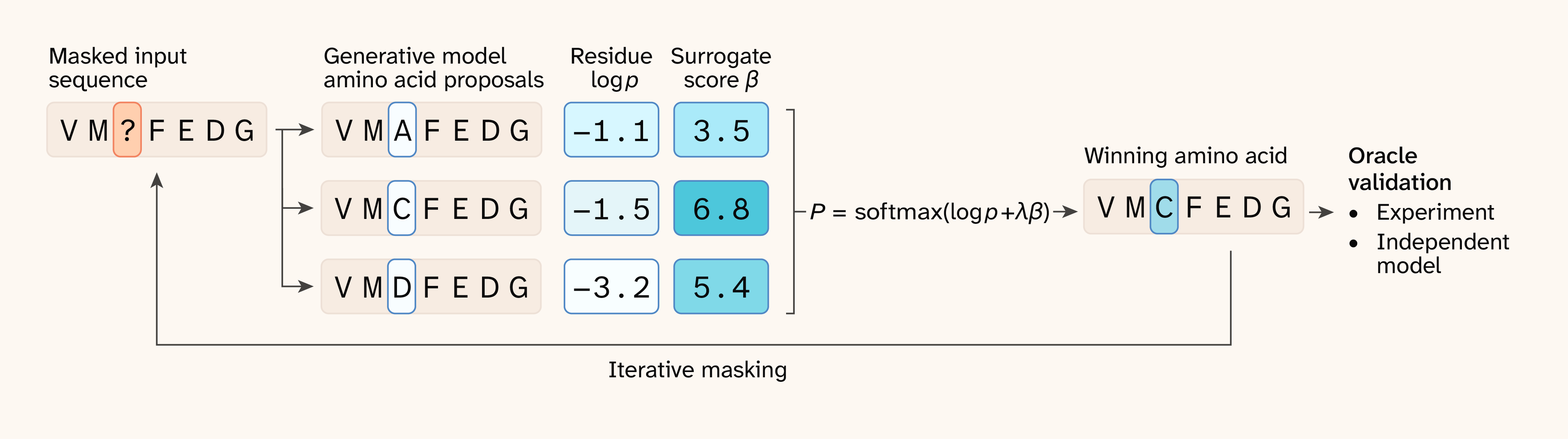
Figure 1. Overview of the property-guided generative design algorithm.
We used iterative single-position resampling as our generative model. At each position, the generative model proposes amino acid priors ; simultaneously, the surrogate model evaluates the sequence property with a score , which can be the distance between the current sequence property from the target. The amino acid is picked based on the softmax probability of the integrated score over top candidates. An oracle — either a separate model or experimental measurements — evaluates the proposed designs.
All associated code, including computational analyses and visualization scripts, and data, including computational results, designed FP constructs, and spectral scans, are available in our GitHub repo (DOI: 10.5281/zenodo.22310324).
FPbase dataset
We curated a sequence-to-peak dataset from FPbase 19 (Figure 2) by retrieving all 1,041 entries (Figure 2, A) via a single GraphQL query. Within each FP family, the emission peaks vary drastically, highlighting the ruggedness of their spectral landscape (Figure 2, B). We applied six successive filters to obtain data entries that are autocatalytically fluorescent with well-defined excitation and emission peaks.
We excluded entries...
- lacking a sequence entirely (51 entries)
- with sequences that contain non-standard or ambiguous residues (X/B/Z/U/O; 14 entries)
- whose chromophore is a bound cofactor, an added fluorogenic dye, or opsin-bound retinal rather than the folded sequence itself (69 entries, matched on name and aliases rather than source organism to avoid false positives)
- without reported excitation and emission maximum for at least one state, which is the operational test for genuine fluorescence (138 non-emissive or erroneous entries)
- representing alternative spectral states of the same sequence, by retaining only the native (bluest) precursor for photoconvertible proteins and the “on” state for photoswitchable proteins (eight entries)
- with no close neighbor in the resulting set (maximum character-4-mer cosine similarity <0.10), since such sequences are unreliable for both training and evaluation (three entries)
This yielded 758 curated sequence–excitation/emission peak pairs (Figure 2, C). In contrast, only 382 pairs passed the filters and reported full spectrum (Figure 2, C). As a result of data availability, we decided to use the excitation/emission peaks to guide the protein design over the full spectrum. A strong positive correlation exists between the excitation and emission peaks in each FP (Figure 2, D), which can also be described as two orthogonal principal components: overall FP color, and its Stokes shift (Figure 2, E–F).
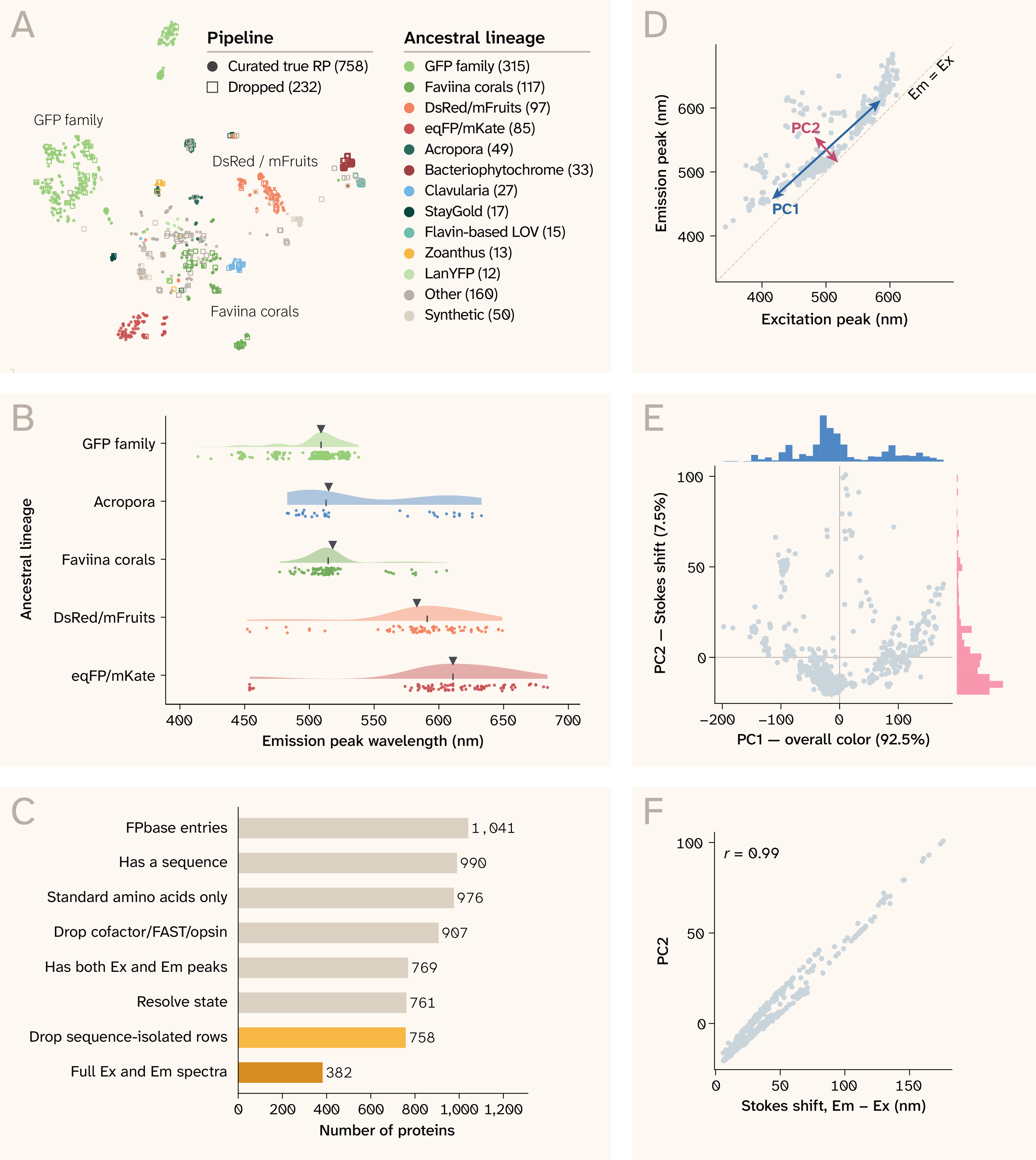
Figure 2. FPbase overview and dataset curation.
(A) FPbase contains 990 sequences belonging to multiple families, shown as the 2D t-SNE embedding of the max-pooled ESM-2 sequence embedding.
(B) The distribution of the emission peak wavelengths for the five most prevalent FP families in FPbase. Triangles mark the founder FPs. Vertical bars mark the family’s median emission wavelengths: GFP family: 509 nm (min-max: 414–538 nm), Acropora/Montipora: 513 nm (483–633 nm), Faviina corals: 514.5 nm (477–606 nm), DsRed/mFruits: 591 nm (452–649 nm), and eqFP/mKate: 611 nm (454–684 nm).
(C) Dataset curation process. From the 1,041 entries, we applied six rules to obtain 758 autocatalytic FPs with well-documented excitation and emission peaks. Only 382 of those entries had full excitation and emission spectra.
(D) Distribution of the excitation and emission peak wavelengths in the curated 758-entry dataset.
(E) Principal component analysis on the excitation and emission peaks reveals two orthogonal directions, with principal component (PC) 1 corresponding to the overall color of the FP, and PC2 corresponding to the Stokes shift.
(F) PC2 aligns with the Stokes shift with Pearson's r = 0.99.
Nested data split
Practically, a protein design campaign using our approach involves two processes: A computational surrogate will steer or filter designs proposed by the generative model, and wet-lab experiments will evaluate the designed sequences. We started off with an in silico test of our algorithm to simulate the real-world use case, replacing the experimental evaluation with an oracle model that scores the resulting designs, held out from the design loop. For the computational proof of principle, we treat the oracle's scores as the decision criterion, the same criterion that the wet-lab experiments will supply. By construction, the surrogate only has partial knowledge of the oracle.
Under this premise, we designed a nested train/validation (val)/test data split to train the surrogate and oracle (Figure 3, A). We first created a random 80/10/10 train/val/test partition over the entire dataset (606/76/76 entries) for oracle training. To simulate the real world, we built the surrogate to be less knowledgeable than the oracle by giving it only a fraction of the oracle's data. We used an 85/15 partition (515/91 entries) of the oracle’s train set with three-fold cross-validation within the 515-entry training set. Both levels are naive random splits with no sequence-identity clustering, related to our use case: We aim to steer a fluorescent protein toward another color, instead of a completely de novo sequence design.
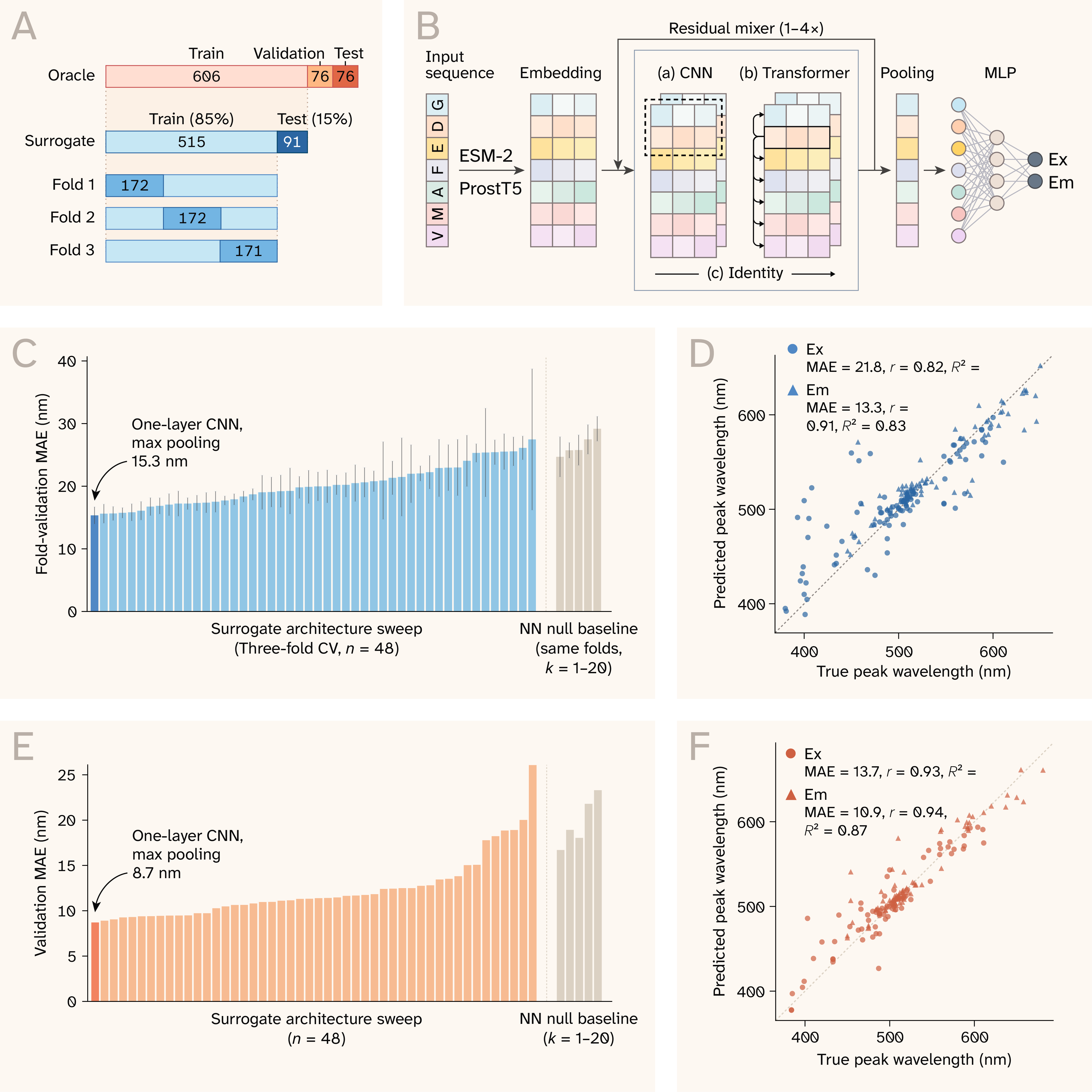
Figure 3. Performance of spectra predictor models.
(A) The nested train/validation/test data split for surrogate and oracle dual model training.
(B) General neural network architecture. We first represent a protein sequence as a residue-level embedding using ESM-2 or ProstT5. We further process the resulting embedding by 1–4 residue-mixing blocks consisting of (a) convolutional neural network (CNN) layers, (b) transformer layers, or (c) no additional processing. We subsequently apply different pooling strategies to generate sequence-level embedding. Finally, a two-layer MLP head operates on the sequence embedding to predict the excitation and emission peak wavelengths (Ex and Em).
(C) Surrogate architectural sweeps, with performance measured by fold-average (mean ± standard deviation [SD], three-fold cross-validation), mean absolute error (MAE) between the predicted and ground truth Ex and Em. The best model (a one-layer CNN that mixes residues on the ESM-2 embedding with max pooling) yielded a mean validation error of 15.3 nm, outperforming null models that predict Ex and Em by the average of nearest neighbors.
(D) Surrogate performance on the test set.
(E) Oracle architectural sweeps, with performance measured by MAE between the predicted and ground truth Ex and Em. The best model (a one-layer CNN that mixes residues on the ProstT5 embedding with max pooling) yielded a validation error of 8.7 nm.
(F) Oracle performance on the test set.
Sequence-spectrum ML model training
Architecture
Both the surrogate and the oracle were lightweight regressors applied to frozen protein language model representations, sharing a single three-stage design (Figure 3, B): a residue mixer, a masked pooling readout, and a supervised head. A protein of length enters as a precomputed per-residue embedding matrix by protein language models (pLM). The surrogate read ESM-2 29 650M per-residue embeddings (layer 33, ), and the oracle read ProstT5 30 encoder embeddings (layer 24, ) to avoid representational blindspots. We padded the embeddings within the batch and created a validity mask derived from true sequence lengths. The residue mixer added context along the sequence axis and took one of three forms: an identity map, a stack of one-dimensional convolution layers (128 channels, kernel width 5, same-padding, ReLU) supplying local windows, or a stack of transformer encoder layers (, four heads, feed-forward 256, dropout 0.2) supplying global mixing, with padding excluded from attention. We then collapsed the mixed representation to a sequence-level representation of the valid residues, using either a parameter-free statistical pool (mean; minimum [min]; maximum [max]; standard deviation [std]; concatenated mean + max + min; concatenated mean + max + min + std), a learned single-query attention pool, or a learned covariance probe that projects each residue embedding to dimensions and captures the uncentered second moment. The supervised head was a two-layer MLP (width 256, ReLU, dropout 0.2) emitting two values rescaled by mean and standard deviation to excitation and emission wavelengths.
Training and architecture sweep
We evaluated the differing architectural designs with the following procedure. We crossed the three architectural axes (residue mixer architecture, depth, and pooling method) into 5 poolings × (1 identity map + 4 convolutional neural networks [CNNs] with different depth + 4 transformers with different depth) = 45 configurations, plus the covariance readout on convolutional depths 1–3, giving 48 configurations per model. We kept channel width, kernel size, head width, attention heads, and dropout fixed throughout. We trained every configuration under one protocol: regression targets standardized on that role's own training fold, mean-squared error in standardized space, Adam optimizer with learning rate 10−3 and weight decay 10−4, batch size 32, and early stopping on validation peak MAE in nm (patience 20, maximum 200 epochs, best weights restored), at a single seed. We ranked configurations by validation MAE; we recorded test MAE for reference only and never consulted it during selection. The single-split surrogate leaderboard proved unstable, so we scored all 48 surrogate configurations by three-fold cross-validation over the pooled surrogate train and validation set (515 entries), with random folds.
Final models
Ranked by the average validation error, one-layer CNN residue mixer and max pooling won at 15.34 ± 1.37 nm (mean ± SD, Figure 3, C). Cross-validation served for architecture selection only, and the deployed surrogate was a fresh refit of winner architecture (one-layer CNN residue mixer and max pooling) on the full 515-entry train and validation dataset, with the epoch count fixed at 71 as the averaged best epochs across the three-fold CV (56/69/88), since no validation data remains for early stopping. On the held-out test set, the surrogate model reached 17.55 nm test MAE (excitation 21.84 nm, emission 13.27 nm, Figure 3, D). We selected the architecture directly from a single sweep of all 48 configurations, with the winner being the same as the surrogate (one-layer CNN residue mixer and max pooling, Figure 3, E) despite using different pLM representations. The oracle attained 8.71 nm validation and 12.27 nm test MAE (Figure 3, F). The oracle is therefore better-informed than the surrogate but not error-free. With the nested training and validation sets, the two models converged to the same architecture.
Nearest-neighbor null model
As a training-free model, we defined a null model that predicts each protein's emission and excitation peaks as the unweighted means of its nearest neighbors’ spectral profiles in the train set, for . We defined the nearest neighbors in the mean-pooled per-residue embedding space (ESM-2 for the surrogate, ProstT5 for the oracle) with cosine distance. We evaluated the null under the same data split as the neural network models by quantifying the peaks based on each validation sequence's nearest neighbors in the train set. Accuracy was best at in every case and degraded monotonically with . Under cross-validation, the surrogate null reached 24.69 ± 3.20 nm (mean ± SD) MAE, higher than 15.34 ± 1.37 nm for one-layer CNN and max pooling during cross-validation. Refit on the 515-entry train set, the null gives 20.08 nm test MAE against the deployed surrogate's 17.55 nm. The oracle null reaches 16.70 nm validation and 18.30 nm test MAE, against 8.71 and 12.27 nm for the selected oracle.
Sequence-brightness ML model training
Deep mutational scanning GFP dataset
In addition to the excitation and emission peaks, we wanted to guide the designs to be viable and bright. We therefore trained a classifier model to provide a bright/dim classification for each design. The bright/dim gate was trained on deep mutational scanning (DMS) data of four green-fluorescent scaffolds: 54,025 avGFP 31 variants 32 and 93,925 variants across amacGFP 33 (35,500), cgreGFP 34 (26,165), and ppluGFP 35 (32,260) 36, 147,950 records in total. We kept records only if they encoded a clean, full-length point-substitution protein with a usable brightness value, excluding those with a premature stop codon, ambiguous residue call, or mutations resulting in C-terminal read-through. We used median brightness of variants of avGFP and the replicate-mean value for the other three scaffolds. We log10-transformed brightness. This yielded 141,144 sequences with recorded brightness: 51,715 avGFP (235 amino acids [aa]), 33,511 amacGFP (237 aa), 24,516 cgreGFP (234 aa), and 31,402 ppluGFP (221 aa). The libraries sit close to their parents with a median of three substitutions, mean of 3.2, and 95th percentile at six mutations.
Every scaffold's log10 brightness distribution is bimodal (Figure 4, A). To make the dataset consistent across the four scaffolds, we took the bright/dim threshold as the lowest-density point between the two peaks of a Gaussian kernel density estimate of log10 brightness (Scott's rule bandwidth, 2,000-point grid). All four scaffolds resolved as bimodal, giving thresholds of 2.41 (avGFP), 3.02 (amacGFP), 3.64 (cgreGFP), and 3.07 (ppluGFP) and bright fractions of 58.2%, 83.5%, 52.8%, and 83.7%. Thus, we transformed log10 brightness to a binary label of bright and dim for the classifier model.
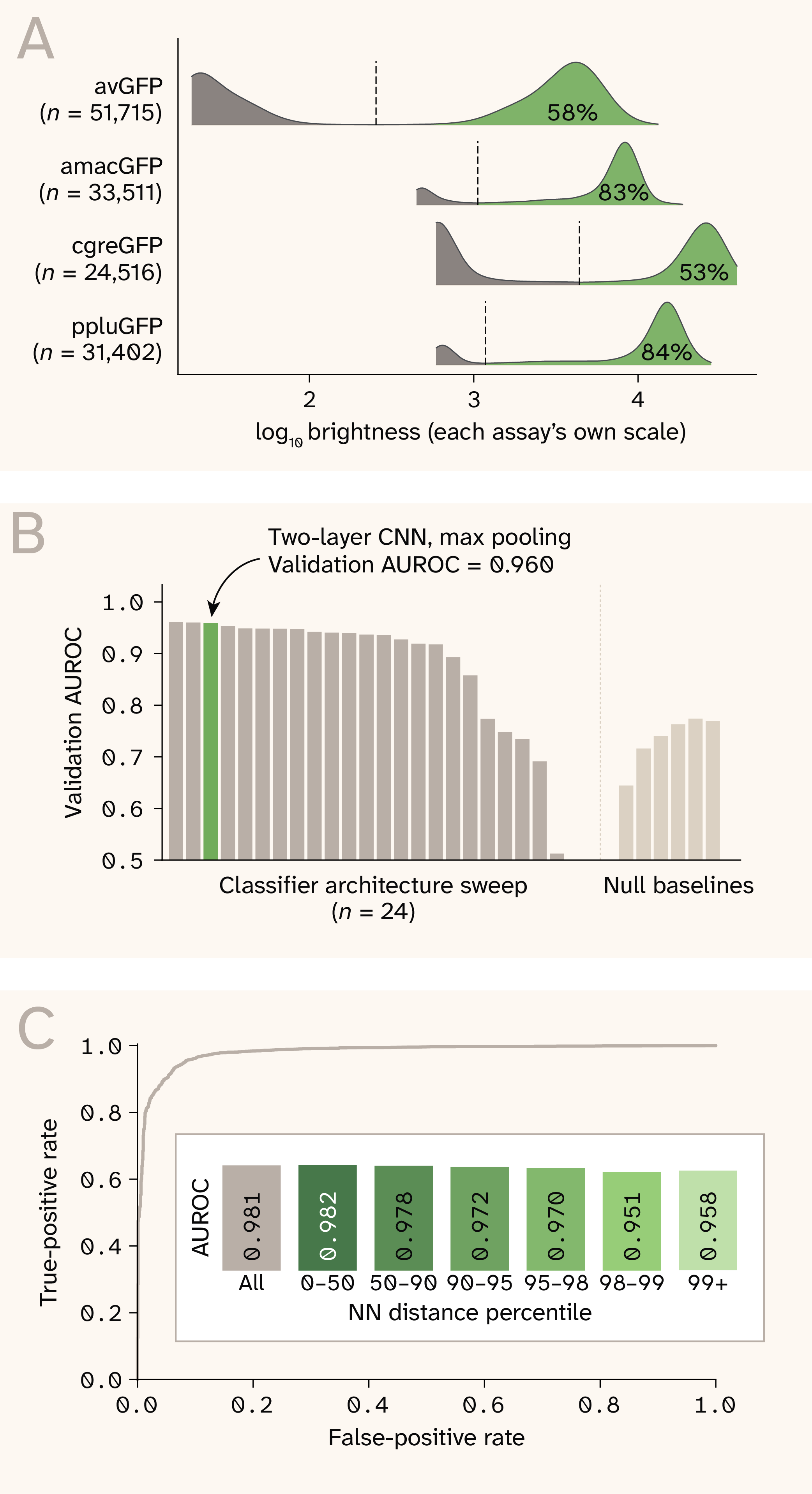
Figure 4. Performance of GFP brightness classifier.
(A) The four GFP DMS datasets all show bimodal distribution in log10-transformed brightness. We took the bright/dim threshold as the lowest-density point between the two peaks of a Gaussian kernel density estimate.
(B) Model architectural sweep. We evaluated model performance using area under the receiver operating characteristic curve (AUROC) on the validation set for each classifier. We picked the two-layer CNN residue mixer model with max pooling over the other two top-performing models, which require more complicated pooling strategies. Null models include -nearest neighbors (cosine similarity) in max-pooled ESM-2 space, a logistic regression on substitution counts, and scaffold identity.
(C) We refit the selected architecture on twice the data of a 10,000-variant-per-scaffold subsample (40,000 total; 28,000 train/6,000 validation/6,000 test, stratified per-scaffold). It reached 0.9816 validation and 0.9809 test AUROC. Inset: Classifier’s performance across nearest neighbor (NN) distance strata in the held-out dataset.
Architecture and training sweep
The classifier reused the three-stage design of the peak models (Figure 3, B): a residue mixer on ESM-2 650M embeddings, a masked pooling readout, and a supervised head emitting a single logit. The sweep grid crossed six pooling readouts (mean; max; concatenated mean + max + min; concatenated mean + max + min + std; single-query attention; and the covariance probe) with an identity mixer or a CNN mixer of depth 1–3, giving 24 configurations. CNNs had a channel width of 128, kernel size of 5, with rectified linear unit (ReLU) activation, and the two-layered supervised MLP head had a width (256) and dropout (0.2), with ReLU activation. We trained every configuration under one protocol (Adam optimizer with learning rate 10−3 and weight decay 10−4, batch size 128, maximum 50 epochs with early stopping on validation BCE and best weights restored). Due to the large dataset size, we used a scaffold-balanced subsample of 5,000 variants per scaffold (20,000 total), with 70/15/15 split per scaffold. We used training loss of binary cross-entropy with logits, and positive weight set to the training dim/bright ratio to counter class imbalance. We ranked configurations by the area under the receiver operating characteristic curve (AUROC) for validation. We also fitted two null models on the same 14,000 training variants and scored on the 3,000 validation variants: -nearest neighbor (cosine similarity) in max-pooled ESM-2 space has validation AUROC 0.644 at rising to 0.774 at ; and a logistic regression on substitution count plus scaffold identity reaching validation AUROC of 0.769.
Final model
The top three architectures from the sweep came as a tie (Figure 4, B): The model with a two-layer CNN with concatenated max + min + mean + std pooling had a validation AUROC of 0.9609, the two-layer CNN with concatenated max + min + mean pooling had a validation AUROC of 0.9601, and the two-layer CNN with max pooling had a validation AUROC of 0.9595. We chose the architecture of a two-layer CNN with max pooling for our final model, refit it on twice the data of a 10,000-variant-per-scaffold subsample (40,000 total; 28,000 train/6,000 validation/6,000 test, per-scaffold stratified), trained under the identical protocol and early-stopped at epoch 34. It reached 0.9816 validation and 0.9809 test AUROC at 93.8% test accuracy (Figure 4, C), with precision of the bright call at 96.6% at the threshold of logit >0 and 97.1% at logit >0.5.
We found that GFP’s brightness rates drop sharply as the mutation distance from the ancestor increases 36. We therefore wanted to determine the classifier’s reliability in the sequence space. In the max-pooled and z-scored ESM-2 embedding space, we first stratified the 40,000 DMS subsamples in the classifier’s training and testing by ranking their nearest-neighbor (NN) distance within the cloud. The NN distance at percentiles 0, 50, 90, 95, 98 and 99 were 2.9, 13.0, 21.4, 24.4, 27.6, and 30.2. For the remaining 97,499 held-out variants (excluded from both the sweep and the final model training), we computed each variant’s nearest-neighbor distance to the cloud and assigned it to the corresponding stratum, giving 42,546/41,912/6,364/4,003/1,438/1,234 variants per stratum. Two variants fell closer to the cloud than any cloud member is to its own nearest neighbor, and were not assigned to a stratum. We then evaluated the performance of the classifier in each stratum based on the held-out variants. AUROC ranged between 0.950 and 0.983, even when the sequences are remote from the major training cloud (Figure 4, C). Thus, we considered the classifier to be reliable when an FP’s distance from the nearest neighbor in the training set was at or below the 99th percentile of the training-set NN-distance distribution.
Property-guided protein design
Generative model
We used a generative model to supply the prior plausibility of a candidate residue . We first used the ESM-2 29 650M model, where we masked the position on the design's current sequence (with existing edits) and took the masked marginal.
We also used a FP family-specific probability model created through multiple sequence alignment (MSA). We aligned the 763 unique sequences (758 in the curated set + 5 without Ex/Em peak labels) of the curated FP set (82 source organisms) with MAFFT (v7.526) under FFT-NS-i (--maxiterate 1000, BLOSUM62, run single-threaded with a fixed seed so reruns are bit-identical), yielding 763 × 1,861 columns of which 233 are core at ≥50% occupancy. We computed per-column amino acid frequencies under Henikoff position-based sequence weights to downweight over-represented clades, resulting in an effective sample size of 272. We derived the weights from the 233 core columns, but read the frequencies off the full 1,861-column alignment, so every scaffold position received a profile regardless of its column's occupancy. We excluded gaps from each column. We intersected each editable position's structural alphabet with the residues present in the aligned column, with the renormalized frequencies being their likelihood . With no pseudocounts, a residue absent from every aligned FP at that column is unreachable.
Structure-informed design window choice
Instead of generating the entire ~230 residues of the FP sequences de novo, we started from a known FP scaffold and constrained the design window to the chromophore and its pocket while keeping the rest of the β-barrel backbone unchanged for two reasons. First, prior works have identified the pocket that provides the immediate environment of the chromophore via polarity, charge, hydrogen bond, and packing as the primary drivers for FP’s spectroscopic function 37–38, whereas the distant mutations mostly support folding, brightness, and stability 39–40. Second, the surrogate was trained on a few hundred FPs and was credible only near that manifold; without these constraints, a non-functional sequence can score well while being out of distribution for the predictor neural network models.
For each scaffold, we aligned the sequence modeled in its experimental structure to the dataset sequence (Biotite [v1.2.0] 41: RCSB fetch, mmCIF parsing, and Smith–Waterman alignment with BLOSUM62 and affine gap penalties −10/−1) and took every residue with a heavy atom within 5 Å of the chromophore. We found the chromophore from both ends: in the sequence as the X-[YWHF]-G motif nearest position 65, and in the structure as the fused non-standard residue those three become on maturation, identified by the gap it leaves in the residue numbering. Because the window is a list of sequence positions, a structure that maps imperfectly yields a silently misnumbered window rather than a noisier one, so we required ≥90% identity over ≥70% coverage and discarded the scaffold otherwise. Chromophore positions 1–2 plus the identified pocket were editable, while we held chromophore position three and the catalytic Arg/Glu pair fixed due to their critical role in chromophore cyclization and maturation. Two positions additionally carried alphabet constraints: chromophore position two stayed aromatic (Y, W, H, F), for its ring bears the conjugated system, and we restricted residues whose side-chain N or O lies within 3.5 Å of a chromophore polar atom to hydrogen-bond-capable residues, so the design wouldn't silently delete the interaction. Overall, we think this represents a structurally plausible and chemically appropriate design space.
Gibbs sampling
We searched sequence space through Gibbs sampling restricted to the per-scaffold design window as described above. We defined a design cycle as one sweep over this window by first visiting the chromophore position and then the pocket in a random order. At each position , we queried a generative model for its conditional distribution over residues ( = 1, 2, …, 20) conditioned on the rest of the current sequence, restricted it to the position's allowed alphabet, retained the top candidates, and sampled one from a softmax at temperature . We updated each position immediately, so every later position in the sweep conditioned on the updated sequence.
Guided design
Guidance entered by re-ranking the candidates before one is drawn. We passed each candidate sequence ( = 1, 2, …, ) to one or a group of surrogate models. We used each model to predict the corresponding property , with indicating a specific property. Each property penalized the sequence by . Candidate amino acid received the composite score , where we z-scored each and to zero mean and unit variance across the candidates. We updated the position by drawing from a temperature-scaled softmax over these scores: , with determining the generation diversity: smaller encourages greedy selection and larger encourages design diversity. In both Gibbs sampling and guided designs, we applied two cycles of sampling for the in silico test, and three cycles for the final EGFP design campaign. Each cycle enumerated the design window with random order. In our designs, we used and .
Experimental validation
We chose ten designs to test in vivo in a pilot experiment, including seven targeting mOrange spectrum, and three targeting blue. We used positive controls of EBFP 42, EGFP 43, and mOrange 20. All constructs were destined for E. coli expression, in a pET28a(+) vector. They all had an N-terminal His tag followed by a Gly-Ser-Gly-Ser linker before the first amino acid of each design. Every design construct used matching codon optimization, except for the sites of mutation, in an attempt to normalize expression. EBFP and EGFP had matching codon optimizations along with our designs, but mOrange did not, since the sequence differs significantly from the others. Finally, we had a negative control of "cells only" in which we transformed an empty vector (pUC19) into BL21(DE3) cells.
We transformed these constructs into BL21(DE3) cells (ThermoFisher EC0114) and picked single colonies into 2 mL LB to grow starter cultures. We grew these in a deep-well 24-well plate at 37 °C, 300 rpm (25 mm orbital shaker), overnight. We then diluted starter cultures 1:200 into 8 mL growth cultures of autoinduction media 44 in flasks. We grew these for 3 h at 37 °C, and then transferred to 25 °C for growth for 48 h, shaking at 200 rpm. We further incubated the cultures at 4 °C for four days to make sure the fluorophores matured properly.
After growth, we measured the OD600 of the cultures and normalized them to the equivalent of 1 mL at OD600 = 6. We then spun down those cultures, washed 1× with PBS, and resuspended the pellets in 60 μL PBS for spectral measurement.
We performed spectral measurements on a Molecular Devices SpectraMax iD5. We took measurements using 50 μL of culture in 384-well plates with black walls and glass bottoms (CellVis P384-1.5H-N). We took spectral scans using the fluorescence feature, fixing an emission wavelength to perform an excitation scan, and vice-versa, with a step size of 10 nm. We set the PMT gain to auto for all measurements. The fluorescence spectra were normalized by subtracting the E. coli pUC19 control and normalized by their maximum intensity.
Computational results
We aimed to computationally test the effectiveness of the property-guided algorithm, and we applied it to try to re-engineer EGFP towards blue and orange spectra.
Spectra conditioning guides FP scaffolds to remote targets
We focus on redesigning the chromophore and its pocket, as they are the primary drivers of excitation and emission spectra. We first tested our pipeline by redesigning the chromophore and pocket of known scaffold FPs to distinct, defined spectra. The surrogate score is the mean absolute error (MAE) between the design’s predicted and the target excitation and emission peaks.
To identify the design window for each scaffold, we retrieved the protein structures from the RCSB Protein Data Bank with ≥97% sequence identity and attempted to align the resolved chain and the sequence. Based on the ≥90% identity and ≥70% coverage criteria, we obtained design windows for 250 scaffolds out of 358 candidates with a potentially matching structure, with 37 sitting inside the surrogate test set. We selected the scaffolds within the oracle train set, but split them by half in the surrogate’s train and test sets. This enables us to evaluate both in-distribution and out-of-distribution designs guided by the surrogate with high credibility from the oracle. We picked 36 scaffolds from the surrogate train set and 36 from the test set. We drew target spectra from real proteins rather than specifying them arbitrarily. This guarantees that every target is achievable by some fluorescent protein and prevents non-existent photophysics. However, this doesn't guarantee the target is achievable from a particular scaffold. We picked scaffolds and their targets with sequence identity between 50% and 98%, within a 30-residue length difference, and with a Euclidean distance of excitation and emission peaks exceeding 40 nm. We randomly drew the target for each scaffold from the qualified candidates.
In this task, we used ESM-2 650M as our generative model. For each of the 72 design pairs, we ran three design trials, each with randomized visiting of the design window. As a benchmark, we also ran unguided Gibbs sampling over the same design window for 12 trials per pair, then scored all 12 designs with the surrogate and kept the top three. Thus, both guided design strategy and post hoc filtering used the surrogate model, and the oracle evaluated the designs. Guided design improved on the unedited scaffold by a mean of 34.5 nm on training (median 23.8, range −8.0 to 118.8; t(35) = 6.74, p < 0.001, paired Cohen's dz = 1.12) and 18.1 nm on testing (median 15.9, range −71.9 to 88.4; p = 0.003, dz = 0.54) (Figure 5, A). Meanwhile, the post hoc filtering strategy improved on the scaffold by a mean of 28.8 nm on surrogate train (median 22.4, range −2.8 to 110.2; t(35) = 6.30, p < 0.001, dz = 1.05) and 9.1 nm on test, which we couldn't separate from zero (median 4.2, range −56.0 to 88.1; t(35) = 1.66, p = 0.106, dz = 0.28).
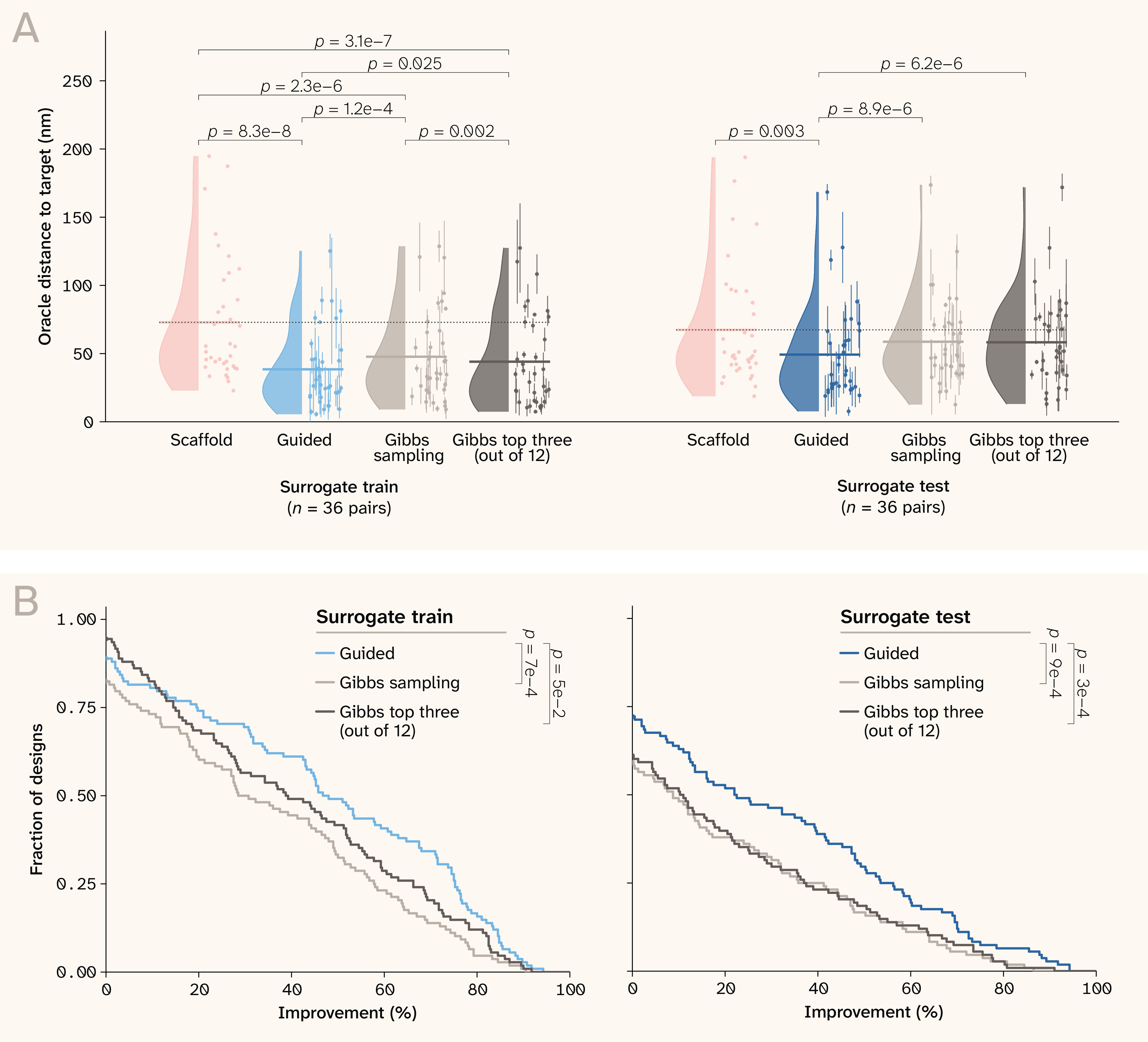
Figure 5. Guided generation moves the FP scaffolds close to their targets.
(A) Distance of the scaffolds and designs (mean ± standard deviation, n = 3 design trials) to the target spectra, evaluated by the oracle. Guided generation (blue) outperformed Gibbs sampling (dark purple) and post hoc filtering strategies (Gibbs top three, light purple), when the scaffolds belonged to both the surrogate train set and test set. We performed paired t-tests to determine the statistical significance.
(B) Fraction of designs (36 pairs × 3 trials per strategy) with different amounts of improvement in spectral distance. Guided designs had the best improvements from the scaffolds out of all three. Two-sample Kolmogorov–Smirnov statistic.
When comparing the guiding and filtering strategies, guidance won by a marginal mean of 5.6 nm (38.4 vs. 44.1 nm; median 2.1, range −16.2 to 46.2; t(35) = −2.35, p = 0.025, dz = 0.39) in the train fold. Although the guidance won on 22 of 36 pairs, the distribution-free Wilcoxon test was unable to separate them (p = 0.088). On the test fold, guided design won by a mean of 9.0 nm (49.3 vs. 58.3 nm; median 8.6, range −15.9 to 28.6; t(35) = −5.31, p < 0.001, dz = 0.89), being closer on 27 of 36 pairs.
We further evaluated the amount of improvement for each scaffold after the design cycles (Figure 5, B). Since the design pairs are variable in their distances between the scaffold and target, we focused on the relative improvement per scaffold. We evaluated each strategy's performance in the train and test sets using survival curves over each strategy's 108 designs (three designs for each of the 36 scaffolds) — the fraction of designs that exceed a given improvement threshold. On training-pool scaffolds, the filtering strategies outperformed the guidance at improvement thresholds below 12%, which for many design pairs is below the oracle’s own uncertainty. Guidance led by six points at 25% improvement (0.70 vs. 0.64), seven at 50% (0.49 vs. 0.42), and by its maximum of 14.8 points at 71%. This suggests the filtering strategy discards failures but doesn't produce large moves, as manifested by the crossing between the two curves. On test scaffolds, guidance led at every threshold: by 11 points at zero (0.72 vs. 0.61), 15 at 25% (0.49 vs. 0.34), and 11 at 50% (0.30 vs. 0.19), with a median improvement of 22.1% against 10.5%. However, neither strategy drew closer than 94% improvement.
Overall, these results highlight that applying the surrogate inside the generative process outperforms using it as a downstream filter, particularly on scaffolds the model was never fitted to.
ESM-2 generates under-specified prior distributions for fluorescent proteins
Single-sequence protein language models (pLMs) generate reasonable priors due to their training across large sequence databases to internalize structural, functional, and evolutionary regularities. On the other hand, models that operate directly on MSAs have shown that family-specific evolutionary information remains a powerful, parameter-efficient alternative 45–46. In our use case, we ask whether ESM-2 has learned the FP family prior well enough to substitute for the information available directly from an FP MSA. To test this, we compared the per-residue log-probability distributions produced by ESM-2 with the position-specific distributions derived from our FP alignment.
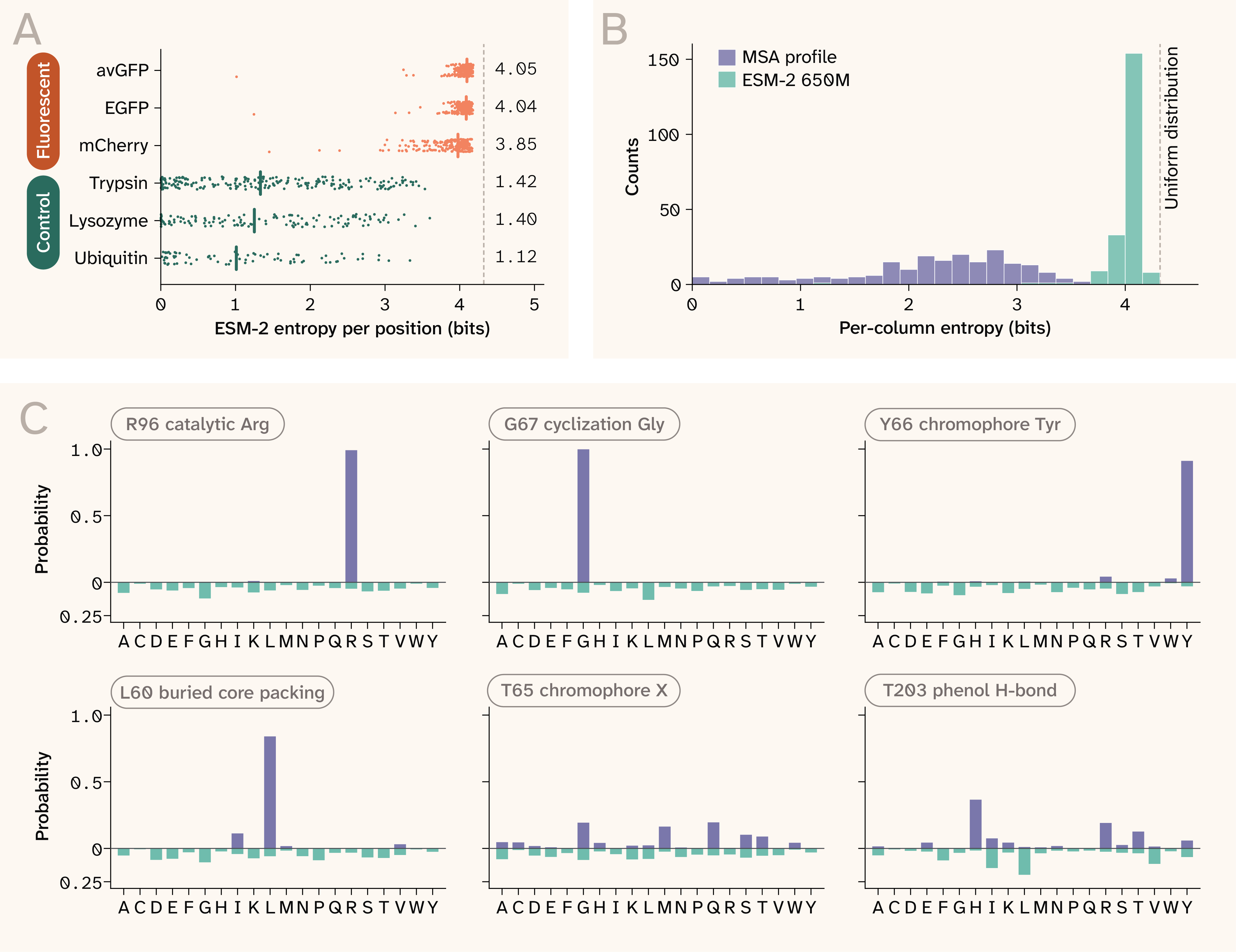
Figure 6. ESM-2 fails to capture the FP family residue profile.
(A) ESM-2 650M masked-marginal entropy at every position of three FPs (orange) and three non-fluorescent control proteins (green). The vertical bars indicate the medians, and the per-protein mean is on the right. Ubiquitin (UniProt P0CG47, 76 aa), lysozyme (UniProt P00698, 129 aa), and trypsin (UniProt P00760, 223 aa) average 1.12, 1.40, and 1.42 bits while mCherry (236 aa), EGFP (239 aa), and avGFP (238 aa) average 3.85, 4.04, and 4.05 bits. The dashed line at 4.32 bits indicates the null model — uniform distribution across the 20 amino acids.
(B) Entropy at each of the 208 columns with occupancy ≥90%. We defined columns by the 763-sequence multiple sequence alignment (MSA). We calculated entropy based on the Henikoff-weighted family frequency (purple) and under the ESM-2 650M masked marginal on EGFP (green). The family's entropy spans the full range, with a median of 2.35 bits (IQR 1.80–2.80); ESM-2's median is 4.09 bits (IQR 4.03–4.13).
(C) Residue frequencies from each MSA profile (purple) against the ESM-2 650M masked marginals (EGFP scaffold, green) at selected positions.
During the masked-residue recovery test, ESM-2 650M had a per-position median entropy of 4.06 bits (IQR 3.97–4.12) for FPs avGFP 31, EGFP 42, and mCherry 20, against a median entropy of 1.25 bits (IQR 0.36–2.21) for other control proteins (Figure 6, A). The null model, uniform distribution across the 20 amino acids, sits at 4.32 bits. In contrast, an MSA-based profile produced entropies with a median of 2.35 bits (IQR 1.80–2.80) (Figure 6, B). At specific locations, the FP family became highly constrained due to their corresponding physicochemical properties, such as the chromophore tripeptide, catalytic residues for chromophore maturation, and wavelength-tuning pocket (Figure 6, C). Across the six example positions on EGFP in Figure 6, C, MSA generated maximum probability with a median of 0.88 (IQR 0.48–0.97); ESM-2 generated almost uniform distributions with a median of 0.11 (IQR 0.10–0.13). These results motivate the use of MSA profiles in place of ESM-2 to propose biophysically plausible generative priors for FP design.
Steering EGFP scaffold toward orange and blue
We attempted to steer the EGFP scaffold toward orange and blue FPs. For the targets, we used the spectra of mOrange 20 and EBFP 42. GFP's chromophore forms autocatalytically from the Thr-Tyr-Gly tripeptide into a p-hydroxybenzylidene-imidazolinone, a single-ring system with a fixed, relatively short conjugated π-electron pathway. As a result, this tripeptide set a redshift ceiling. EBFP 42 differs from EGFP by two point mutations 43, 47: Y66H replaces the chromophore phenol with an imidazole, shortening the conjugation π system and blue-shifting the spectra to ~380/440 nm 48, and Y145F partially offsets the accompanying loss of quantum yield 42. On the other hand, the GFP scaffold is capped at yellow due to the biophysical constraint in its chromophore. On the β-barrel pocket, T203Y introduces an aromatic side chain that π-stacks against the chromophore's phenolate ring, polarizing its excited state and nudging emission toward yellow without altering the chromophore's underlying structure 49. Engineered orange proteins 20 were based on DsRed-type chromophore, which extended the ring system through an N-acylimine bridge to further involve the carbonyl of Phe65 50. The mOrange series blueshifted from red through a Q66T substitution that attacks the carbonyl carbon of Phe65, so the conjugation system gets shortened 51. Therefore, designing toward blue represents an easier target for our campaign, while orange is harder. We enabled modifications to both the chromophore and its surrounding pocket in our design window.
For a protein to function properly, it needs both optimized functionality and viability, as determined by expressibility, solubility, and foldability. A protein predicted to have target functionality isn't guaranteed to be viable. In the current property-guidance framework 15, this multi-objective optimization is technically achievable yet rarely considered. On top of the spectrum predictor (Figure 3, D), we further included a brightness classifier (Figure 4, C) in the campaign based on four GFP deep mutational scan (DMS) datasets 36 using brightness as a proxy for viability. This bears an important caveat: in these datasets, the protein brightness was quantified at defined excitation and emission wavelengths in the green channel. Since our designs target other colors, the classifier is supposed to rate the spectral cross-talk. Despite this caveat, we think protein brightness is a sufficient proxy for protein viability. As a result, a design classified as bright should, in principle, be viable with green-channel emission bleed-through. In the DMS dataset, since the variants’ bright rates drop sharply with increasing mutation distance 36, and to also constrain the designs within distribution for the brightness classifier, we further included a penalty on the number of edits allowed. As a result, at a given position, the score of residue becomes:
Here, and are the surrogate-predicted excitation and emission peak wavelengths, and are the target excitation and emission wavelengths, is the raw logit by the brightness classifier, and penalizes a change from the original residue and if the original residue is .
| Strategy | Generative prior | Trials/combination | Total designs | |||
|---|---|---|---|---|---|---|
| (1) ESM-2 Gibbs | ESM-2 650M | 0 | 0 | 0 | 375 | 1,125 |
| (2) Spectra guide | ESM-2 650M | 0.25/0.5/1/2/4 | 0 | 0 | 75 | 1,125 |
| (3) Spectra + brightness guide | ESM-2 650M | 0.25/0.5/1/2/4 | 0.5/1/2/4 | 0/0.5/1/2/4 | 4 | 1,200 |
| (4) MSA guide | MSA | 0.25/0.5/1/2/4 | 0/0.5/1/2/4 | 0/0.5/1/2/4 | 12 | 4,500 |
| (5) MSA Gibbs | MSA | 0 | 0 | 0 | 375 | 1,125 |
Table 1. Hyperparameter combinations, and number of designs proposed for each design strategy to steer EGFP toward orange and blue spectra.
We tested two generative priors (ESM-2 and MSA profiles) in combination with various design strategies (Gibbs sampling and post hoc filtering, spectrum guidance, spectrum and brightness guidance) with different combinations of hyperparameters (Table 1). Across the hyperparameter combinations, we ran each strategy for three trials, each with three optimization cycles, yielding ~1,125 designs per target. Since the unguided Gibbs sampling strategy ((1) and (5) in Table 1) is target-agnostic, we used the same 1,125 designs for the two targets for comparison. In the absence of any guidance, Gibbs sampling with an ESM-2 prior generated zero designs that are in-distribution for the brightness classifier (Figure 7, A). Here, we define in-distribution as the sequence’s distance from the nearest neighbor in the training set being within the 99% strata of the training set. In contrast, since the MSA profile constrained the candidate residues, Gibbs sampling with the MSA prior generated 100 in-distribution designs (8.9%). When we did not use brightness to guide the generation process (Gibbs sampling and spectrum-only guidance), the brightness classifier predicted zero designs to be bright (with logit >0.5). In the absence of brightness classifier guidance, these designs have, on average, 20.7 ± 2.6 (mean ± SD, n = 4,494) mutations (min-max = 11–25). In comparison, the DMS variants lost their brightness beyond 3–7 mutations 36. As a result, these designs are out of distribution from the DMS variants, and largely not expected to be bright in the green channel. This highlights the challenge of low hit rate with the post hoc filtering strategy.
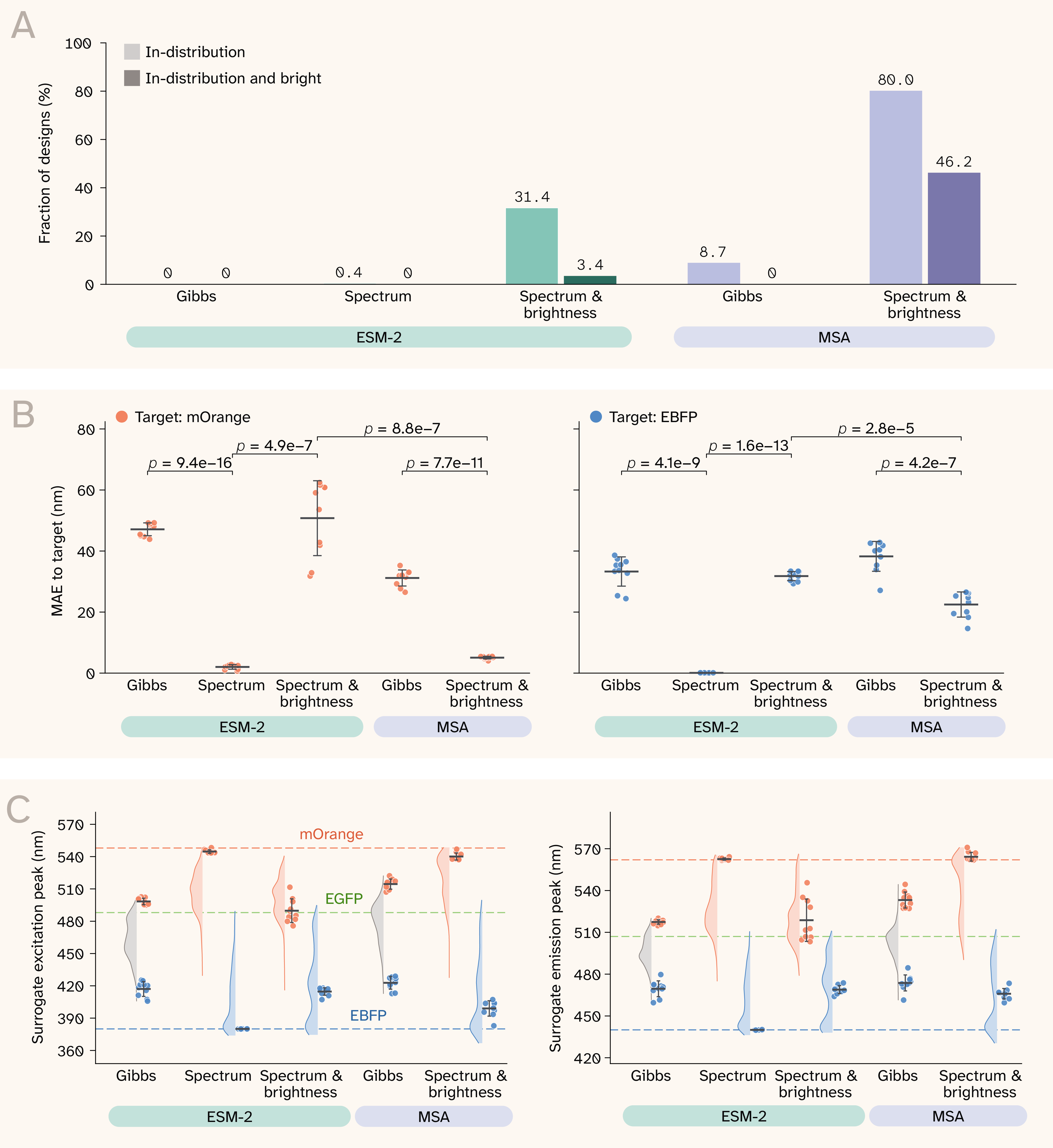
Figure 7. Re-designing EGFP for alternative spectra.
(A) Out of the ~1,125 per design strategy, fractions of designs that are in-distribution of the brightness classifier (light shade), and also predicted to be bright (dark shade).
(B) MAE distance of the top 10 designs of each strategy to the target mOrange (left) or EBFP (right) spectra, evaluated by the same surrogate model that guides the generation. Bars represent the average across the 10 designs with one standard deviation (SD) whiskers. Welch’s t-tests (two-sided) were performed to determine the statistical significance.
(C) Surrogate-predicted excitation and emission peak wavelengths for the entire ~1,125 designs (KDE distribution) and the top 10 designs for each target. Scatters represent the individual designs, bars represent the average across the 10 designs with one SD whiskers. The EGFP scaffold, and mOrange and EBFP target spectra are shown in colored dashed lines.
For mOrange as the target, we generated ~1,125 designs for each strategy (Figure 7, B–C). We picked the top 10 designs ranked by the MAE between the predicted and target excitation and emission peaks. For the spectrum- and brightness-guided strategies, we applied an additional filter so the designs would be in-distribution and predicted to be bright. With ESM-2 as the generative prior, designs conditioned only on spectrum were MAE = 2.01 ± 0.75 nm (mean ± SD, n = 10) away from the target (Figure 7, B), however, the brightness classifier predicted none of them to be bright. With the brightness guidance, bright designs and orange designs exist, but they don’t overlap. As a result, the top-performing bright designs have spectra that are remote from the target 31.16 ± 2.64 nm (mean ± SD, n = 10, Figure 7, B). When using MSA as the generative prior, and spectrum and brightness as the guidance, the top 10 bright designs got closer to the target, with MAE = 5.07 ± 0.43 (mean ± SD, n = 10, Figure 7, B).
We originally considered EBFP to be a comparatively easy target: it has only two mutations compared to the EGFP scaffold, and both positions are within our design window. Surprisingly, among the strategies we tested, only spectrum-based guidance generated designs 0.07 ± 0.04 nm (mean ± SD, top n = 10, Figure 7, B) away from EBFP, yet the brightness classifier classified none of the designs as bright. The dual-guidance strategies were able to generate designs that were either bright or close to the EBFP spectrum, but not both. Nonetheless, the bright designs still have predicted emission wavelengths of 468.9 ± 2.9 nm (mean ± SD, n = 10, Figure 7, C) for ESM-2 prior, and 465.9 ± 3.7 nm (mean ± SD, n = 10, Figure 7, C) for MSA prior, within the blue channel and leaning toward cyan.
We also evaluated the sequences of EBFP and mOrange with the brightness classifier and found both predicted to be dim. EBFP is only four mutations away from avGFP and is in-distribution for the classifier. However, it’s predicted to have a logit of −3.76. Spectrally, avGFP brightness was measured in the filter of 510/30 nm (495–525 nm) in the DMS dataset. Within this range, the fraction of emitted photons for EBFP is 0.077, in comparison to 0.572 for avGFP. Moreover, the molecular brightness for EBFP was weaker than avGFP (4,930 against 19,750). As a result, EBFP’s intensity within this range was ~29.9× weaker than avGFP. Therefore, there’s barely any cross-talk of EBFP in the green channel, potentially explaining the classifier’s failure to identify it as bright. mOrange originated from DsRed and is therefore out of distribution for the GFP brightness classifier. Spectrally, the fraction of emitted photons within the 495–525 nm range was less than 0.012, and its intensity was more than 20× weaker than avGFP. The minimal spectral bleedthrough potentially explains the design’s trade-off between the classifier’s brightness and spectral distance from the target.
Experimental results
Strategy (4) uses the MSA profile as the generative prior and guides the generation with both the spectra predictor and brightness classifier. We found that this strategy performed best across all strategies, computationally. We thus expanded our design pool of this strategy by running nine additional trials per hyperparameter cell, ultimately yielding 4,500 designs. Among these designs, we selected five designs that were in-distribution for the classifier, predicted to be bright (logit >0.5), and ranked the closest to mOrange, and three designs closest to EBFP. We also picked two designs predicted to be closest to mOrange from MSA-Gibbs strategy, but didn't require them to pass the brightness classifier. We experimentally tested the 10 designs by transforming the plasmids into E. coli and measuring their corresponding spectra.
Based on plate reader measurements, we only saw fluorescent signals from one of our ten designs. The bright design was guided by the algorithm toward orange. Our preliminary data suggests that our nine designs failed due to solubility and folding issues, but we need to further investigate to be sure. The bright design fluoresced in the green channel (Figure 8) instead of orange, with two excitation peaks at 390 and 500 nm, and one emission peak at 520 nm. The scaffold EGFP had measured peaks at 490 nm excitation and 520 nm emission, in agreement with the reported 488/507 peaks 43. The guidance targeted the 548/562 nm excitation/emission peaks of mOrange 20.
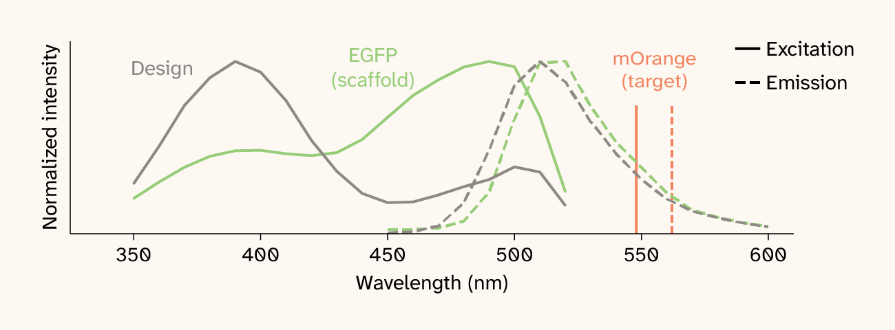
Figure 8. Fluorescence spectrum of the bright design.
Fluorescent spectral scan of the bright design and EGFP. The excitation spectrum (solid curve) was measured with fixed emission wavelength of 560 nm, and the emission spectrum (dashed curve) was measured with fixed excitation wavelength of 390 nm. The vertical, orange lines correspond to the target excitation and emission peaks of mOrange the design was guided toward.
The design carries six mutations from the EGFP scaffold. Here we report them in conventional avGFP numbering: F46L, L64F, T65M, V68S, Y145F, T203H. Among these mutations, T203H places an aromatic imidazole at the position that stacks against the chromophore phenolate, mimicking T203Y in YFP 49. F46L is the same mutation as part of Venus' fast-maturation mechanism 52 that accelerates chromophore oxidation. L64F reverts EGFP’s F64L, which improves folding efficiency at 37 °C 53. F64 is found in multiple orange and red FPs, and may thus reflect a statistical pattern of red-shift. The combination of L64F and T65M reconstitutes mCherry’s chromophore-forming motif, an MYG chromophore preceded by Phe64. However, mCherry’s acylimine-forming oxidation that red-shifts the spectrum requires catalysis by Lys70, the chemistry absent from the GFP scaffold. These results suggest the surrogate model has learned a mixture of statistical patterns and partial biochemistry that predicts existing FPs accurately but transfers across lineage boundaries poorly. As the design is a combination of DsRed lineage chromophore and GFP β-barrel, the predicted hit on orange spectrum could be an extrapolation of the surrogate model.
Discussion
In this work, we applied a multi-property guiding framework to sample sequence space to find protein design candidates with multiple desired properties. Using FPs as an example, we built predictor models of FP spectrum on the small FPbase dataset 19 and of brightness on larger GFP DMS datasets 32, 36. FPs provide a useful test case for the availability of sequence–phenotype datasets, their broad applications, and the ease of measuring spectral properties. However, an FP is also a self-modifying protein: it autocatalytically forms its own chromophore, coupling sequence design to chemical reactions 54. While the guidance algorithm appeared computationally effective, the experimentally measured phenotypes did not shift toward the guided target. Several non-mutually-exclusive factors could explain this discrepancy. First, the orange spectrum may be poorly accessible from the EGFP scaffold. Our fixed EGFP β-barrel may not allow the maturation of an orange chromophore. Second, our design window — the chromophore and its pocket — controls the fluorescence color and is also the most fragile part of the protein, which easily can easily lose its functionality with only a handful of mutations across the entire sequence 5, 36. Aggressive engineering in this focal region can disrupt the pocket geometry that restricts chromophore motion and maintains conjugation. Loss of this rigidity opens alternative pathways for energy dissipation, reducing or abolishing fluorescence. Third, the predictive models could have operated out-of-distribution, rendering our predictions of the designs being bright and orange unreliable. These possibilities point to several potential improvements that could help if we were to reimagine this project, and may serve as generalizable takeaways for others embarking on protein design efforts.
First, design campaigns should treat the choice of starting point as part of the optimization problem instead of a fixed prerequisite. Whether the initial state is noise with imposed symmetry 1, a functional motif 5, a set of constrained residues 5, or an existing candidate sequence, it defines the region of sequence space that the design procedure can effectively sample. Because the sequence–function landscapes are rugged and only sparsely measured, practical designs tend to be confined to the local optima. Identifying an evolutionary precedent or deliberately redesigning the starting scaffold 55 may therefore define a better search space and improve the accessibility of the target phenotype.
Second, if we revisit this, we want to leverage the existing dataset and create our own in a more informed manner. We initially treated DMS-derived brightness as an integrated proxy for biophysical viability, reasoning that variants that fail to fold, mature, or express would lose their fluorescence. However, brightness is not a pure viability label: spectral shift can reduce the signal in the green channel even when the protein remains fluorescent. More importantly, the training and design distributions differed structurally for our brightness classifier. Error-prone PCR created variants with mutations distributed throughout the entire GFP sequence, whereas our designs concentrated the design window in the chromophore and its immediate pocket. A classifier trained on the former distribution therefore had little guarantee of calibrated performance on the latter. This distribution shift was further obscured by our out-of-distribution metric. The combination of the max pooling strategy and ESM-2’s lack of knowledge towards FPs retained too little positional information to distinguish between globally distributed mutations and pocket-concentrated ones. We see several ways out: (1) filtering the DMS dataset to focus on the chromophore-concentrated mutants, (2) experimentally performing local DMS on the chromophore and its pocket, or (3) potentially creating a universal protein viability model. The third option would be a valuable derisking asset for many protein design efforts. Although individual DMS studies define fitness differently 56, shared signatures of folding, stability, expression, and function integrity may permit general-purpose models to learn the transferable components of protein viability. Alternatively, one can also train property- and sequence-space-specific models leveraging multiple datasets to guide the generation process 57. Another critical consideration in leveraging published datasets is that many existing datasets are a collection of local optima. FPbase is strongly enriched for evolutionary or engineering successes and densely records functional endpoints, but sparsely samples the low-fitness intermediates separating them. A predictor trained on such data may interpolate well with each known FP family but provide poorly calibrated guidance along trajectories connecting distinct optima, leading the design astray. This exposes a fundamental tension in model-guided protein design: Successful generation requires novelty, but novelty itself can invalidate the models used to evaluate it. Addressing this tension requires methods that distinguish useful novelty from unsupported extrapolation: for example, through calibrated, design-aware uncertainty estimates, OOD detection, or generative priors that constrain optimization to regions where phenotype predictions remain reliable.
An additional observation was the surprisingly weak family-specific constraints ESM-2 supplies for FPs. pLMs trained on large collections of natural protein sequences learn statistical regularities that reflect, among other factors, evolutionary and biophysical constraints. Consequently, they can provide a prior that favors sequence patterns resembling those observed in natural proteins. However, because many FPs are engineered derivatives rather than natural homologs, their sequence statistics may differ from those emphasized during pLM training. In contrast, others used ESM3 to design a viable GFP protein that’s only 58% identical to avGFP 5. Despite heavy prompting and active learning, this success potentially indicates its familiarity with the FP family. Understanding and benchmarking the performance and confidence of pLMs across protein families could inform model selection for a particular design campaign. On the other hand, MSA profiles 46, 58 enabled parameter-efficient models with better contact and fitness predictions than single-sequence models. For FPs, our results suggest the MSA-derived profile may provide a better family-specific prior, defining a better biophysically constrained sequence space, enabling effective property-guided searches.
Overall, we've presented a high-dimensional, multi-property-guided protein design strategy with baked-in biophysical and evolutionary information. This guidance framework is generalizable to other proteins, especially when the design objective includes multiple properties or high-dimensional phenotypes. However, based on our experimental data, we warn against the danger of the designs wandering off the supervised models’ distribution and generating false positive signals. We'd love to hear about how our work influences your strategy to model or design your favorite proteins, what their high-dimensional phenotypes look like, and we welcome any suggestions for biophysical/algorithmic improvements of our framework!
Additional methods
We used ChatGPT (GPT-5.6 Sol) to suggest papers on relevant science (we did further reading and cited some of this literature), clarify and streamline text, suggest wording ideas, write text, reorganize text to fit the structure of one of our pub templates, copy-edit draft text to match Arcadia's style, and expand on summary text that we provided. We used Claude (Opus 4.8 and Opus 5) to help write, clean up, comment, and review code, interpret data, suggest papers on relevant science (we did further reading and cited some of this literature), clarify and streamline text, write text, suggest wording ideas, reorganize text to fit one of our pub templates, expand on summary text that we provided, copy-edit draft text to match Arcadia's style, and generate figure mockups.
Chatting with Claude made us realize that ESM-2 is unopinionated about fluorescent proteins, which inspired us to leverage family MSA profiles as an alternative prior for protein design. Claude also helped us think about our designed sequences and predict likely mechanistic consequences of the mutations. We reviewed all AI-assisted content and take responsibility for its accuracy and integrity.
We used arcadia-pycolor (v0.8.0) 59 to generate figures before manual adjustment.
Acknowledgments
We'd like to thank Ilya Kolb for early microscopy work that we didn't end up including here. Thanks also to Evan Kiefl, Rahul Khorana, James Golden, and Austin Patton for helpful discussions.
Be the first to comment on this publication.