Purpose
Raman spectroscopy is an increasingly valuable tool for interrogating the chemical structure of unknown biological samples 1–4. Simulated Raman spectra complement experimental measurements in terms of screening and interpretation, letting us map spectral peaks to specific molecular bonds and to assist in discerning whether a noisy measured peak is evidence for one type of molecule or another. Density functional theory (DFT), the standard computational approach for generating simulated Raman spectra, is prohibitively slow for larger molecules relevant to biology and drug discovery.
Machine learning approaches, specifically graph neural networks (GNNs) trained on chemical structures, offer an alternative path to efficiently predict simulated Raman spectra for small molecules with reasonable accuracy 5–6. GNNs like DetaNet and Mol2Raman have been trained and evaluated primarily on small-molecule benchmarks, so we wondered whether this approach could generalize to larger drug-like molecules and peptides.
We developed SpectraLoRA, an expanded and post-trained DetaNet GNN architecture, that predicts Hessians, vibrational frequencies, and Raman spectra directly from 3D atomic coordinates. SpectraLoRA extends Raman prediction from small molecules to short peptides and drug-like compounds. We further demonstrate a post-training alignment strategy that improves the prediction of experimentally collected spectra with the RamanBiolib dataset, bridging the simulation-to-experiment gap without requiring large-scale experimental training data.
These results may be useful to those interested in applications of machine learning to molecular representations and spectroscopy.
Background
We investigate the vibrational structure of molecules using Raman spectroscopy. To give a simplified perspective, the measured spectrum from inelastic scattering of single-frequency laser illumination serves as a molecular fingerprint: peak positions indicate approximately which bonds are present, and peak intensities roughly reflect how readily the electron cloud deforms during each vibration. Each energy shift approximately corresponds to a specific molecular vibration, a bond stretching, or bending at a characteristic frequency, dependent on the structure and atomic composition of the sample (in addition to other environmental conditions) 1, 7.
We wanted to build a GNN to predict simulated Raman spectra from molecular structures for drug-like molecules and short peptides, and to adapt it to experimental spectra. Given that Raman spectrum intensities in both simulated and experimental spectra can be somewhat noisy, our initial target was to predict vibrational peaks in spectra.
We wrote this pub for those without an ML background who are interested in Raman spectra prediction. We have tried to summarize the key takeaways in the box below.
Significance for spectroscopists
Why simulate spectra? Experimental spectral databases and reference tables can tell you which peaks are present in a known compound, but not always what those peaks mean in the context of your molecule of interest. Simulated spectra fill several gaps that experimental references alone cannot:
- Simulations allow you to assign peaks to specific vibrational modes
- Simulations can uncover diagnostic peaks that differentiate similar molecules.
- Simulations offer a preview of what a compound's spectrum might look like in the absence of experimental data.
What we built. We trained SpectraLoRA, a graph neural network (post-trained DetaNet architecture) that predicts Raman spectra directly from a molecule’s 3D structure. To generate training data, we used density functional theory (DFT) simulations for drug-like molecules and short peptides (as well as machine-learning approximations of DFT in some cases). DFT remains computationally infeasible for larger biomolecules like proteins, which is why a learned machine learning model for fast inference could be useful. A GNN approach that generalizes from peptides to proteins could eventually provide simulated reference spectra at scales where physics-based simulation simply cannot go.
The catch, and our solution. A persistent challenge for any computational method is that simulated spectra do not perfectly match experimental measurements. This gap matters when real spectral differences carry biological meaning, as our phylogenetic work demonstrates 4. To close this gap, we developed a post-training alignment step that uses a small set of experimentally collected Raman spectra to shift the model’s predictions toward real-world experimental measurements from RamanBiolib 8. This means that as we collect and share more experimental Raman data, we can progressively calibrate the model without retraining from scratch.
The ultimate goal. We'd like to use SpectraLoRA for a future model where we reverse the direction of inference. Because the model is trained on DFT data, it learns a physics-informed internal representation that maps molecular structure to spectra through actual vibrational properties. We plan to build a decoder that runs inference in the opposite direction, predicting molecular properties like mass and hydrophobicity from spectra of unknown samples.
Try it! For biochemists using Raman to characterize pure compounds, SpectraLoRA offers a path toward fast, computationally cheap spectral prediction that complements experimental workflows. Check out our GitHub README to try it yourself. You can run the model in this notebook.
For technical readers, jump straight to our findings, or read on for the methodological details of our approach.
The approach
Others have used graph neural networks to predict Raman spectra because they operate directly on atoms as nodes and bonds as edges, and can learn associations between chemical features and vibrational modes 9–10. As a starting point, we chose the pretrained DetaNet architecture 5, which predicts quantum-mechanical properties of molecules from 3D atomic coordinates. DetaNet has demonstrated strong performance in predicting Raman spectra for small-molecule benchmarks, making it a natural starting point for an extension to peptides and drug-like compounds. DetaNet's particular architecture makes its predictions invariant to rotation and translation of the molecular structure. To scale up DetaNet for the prediction of spectra for larger molecules, we focused on broadening the training set to include larger molecules, expanding the atomic embedding layer and improving the correspondence of predicted spectra to experimentally measured spectra.
Assembling a dataset of larger molecules
We assembled a dataset including the SPICE 11, NABLA2DFT 12, QM9 13, DES5M 14, Raman ChEMBL 15, QMugs 16, Mol2Raman 17, and QM7 18 chemical datasets, which provide molecular energies, forces, dipole moments, and polarizability tensors. SPICE contains small molecules, dimers, dipeptides, and solvated amino acids. We used Raman ChEMBL as a held-out test set, as it consists of peptides containing ≤ 100 atoms not included in the original datasets. The training set includes, as its largest molecule, cyclosporine A, which contains 11 residues and 196 atoms.
Model architecture
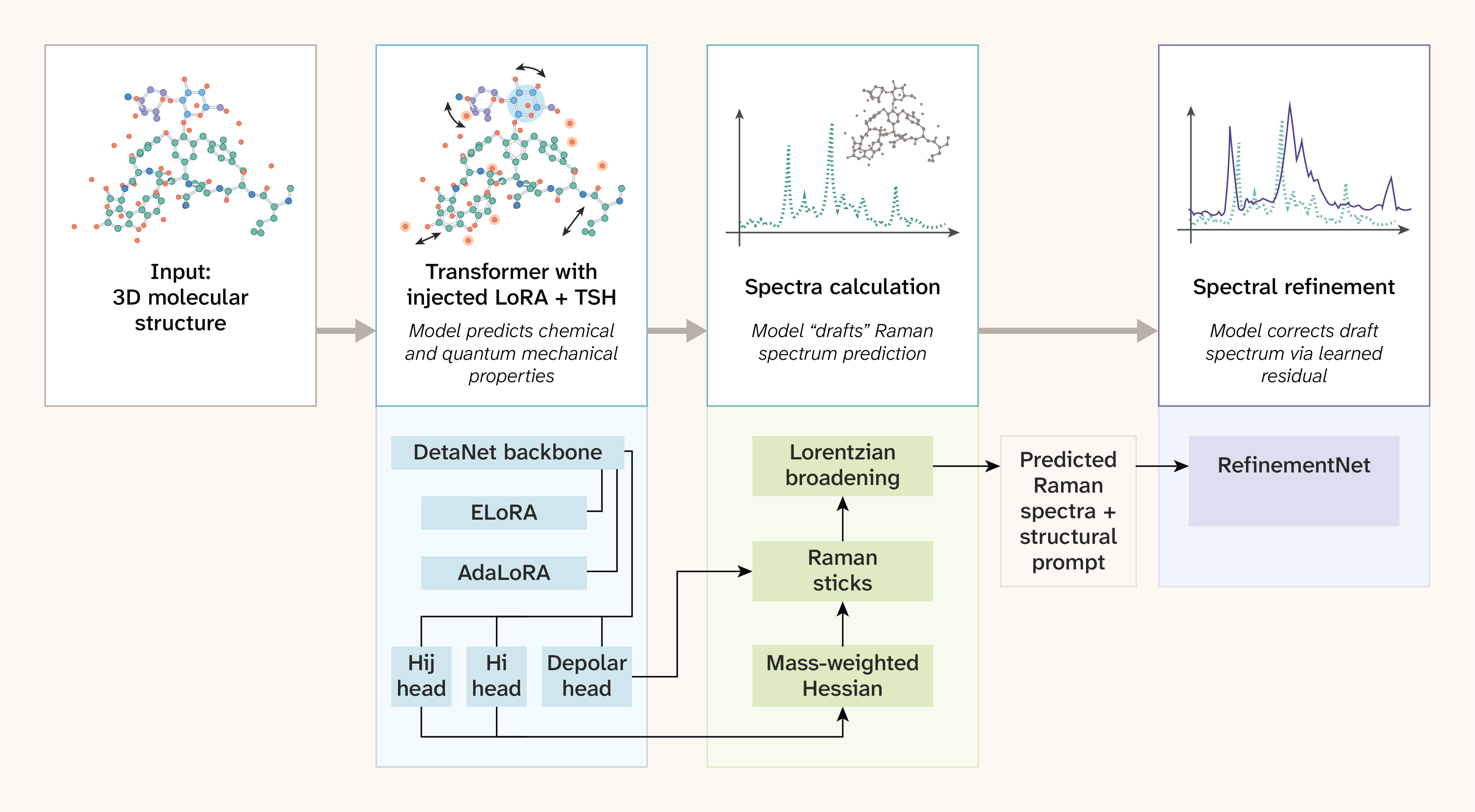
Figure 1. The DetaNet backbone with equivariant tensor-attention blocks produces per-atom scalar and tensor features 5.
Task-specific heads predict molecular Hessian diagonal (Hi) and off-diagonal (Hij) blocks via autograd, plus polarizability derivatives (depolar) via an equivariant head. Based on molecular structure, the pipeline assembles, mass-weights, and diagonalizes the Hessian to yield vibrational frequencies and normal modes; Raman activities follow from the chain rule (see "Task heads and Raman reconstruction"). AdaLoRA (adaptive low-rank adaptation) augments invariant layers while ELoRA (equivariant LoRA) adapts equivariant layers, keeping the backbone frozen.
We fine-tuned the AdaLoRA and ELoRA layers in a supervised fashion on the outputs of the individual task heads using representations from DFT (or an approximation), which produces reasonably accurate predictions for Raman spectral peak locations. We carry out post-training alignment to improve spectral intensity prediction in two phases: Phase 1 trains a 1D U-Net refinement network with structural prompting (FiLM conditioning on Morgan fingerprints) using the peak-weighted RMSE objective of Sorrentino et al. 19; phase 2 hill-climbs the decoder weights via natural evolution strategies 20 to maximize the non-differentiable F1 proxy metric directly.
SpectraLoRA architecture
SpectraLoRA uses the DetaNet equivariant tensor-attention architecture and a subset of the pretrained weights (we discarded some input layer pretrained weights) 5. The architecture is summarized in Figure 1.
Embedding
DetaNet was originally trained on QM9, a benchmark dataset of small organic molecules containing only C, H, O, N, and F, and its embedding layer was designed only to represent those five elements 21. We extend the nuclear embedding table to the full periodic table (Z ≤ 118): We preserve pretrained weights for known elements and initialize new elements with small random values and a fixed electronic configuration feature encoding orbital occupancy (number of s/p/d/f electrons per shell). These architecture alterations allow SpectraLoRA to process arbitrary molecules, including drug-like compounds containing S, Cl, Br, P, and Se in our evaluation set, without retraining the linear layers that comprise DetaNet’s backbone.
Molecular structure representation
SpectraLoRA initially encodes each atom as a node in the molecular graph with its atomic number and electronic configuration. It updates the representations through successive interaction blocks in which atoms exchange information with their neighbors via distance-modulated attention. It preserves 3D rotational symmetry of the representation through equivariant tensor operations. The resulting per-atom features feed into three task-specific heads that predict the molecular Hessian (whose eigenvalues yield vibrational frequencies) and polarizability derivatives (which determine how strongly each vibration scatters light). SpectraLoRA then reconstructs the Raman spectrum from these quantities via matrix diagonalization and the chain rule, rather than regressing them directly 22. The subsequent collapsed section covers the mathematical details.
See details for ML practitioners.
Initialization
The model initializes each atom as:
where is a learnable Swish activation, , with learnable per-channel parameters and .
Tensor-attention blocks
The model maintains two coupled feature streams: invariant scalar features and equivariant tensor features carrying irreducible representations (1,920 components total), where , using interaction blocks with eight attention heads.
Interaction block
Each block performs edge-attention message passing followed by equivariant self-attention. For edge with distance and direction :
Message phase
Scalar features produce queries, keys, and values via linear projections. Keys and values are modulated by trainable Bessel radial basis functions :
The edge feature is split into a scalar message and a tensor-product input , which is coupled with spherical harmonics via a Clebsch-Gordan tensor product:
Update phase
The model sums messages over neighbors and adds them via residual connections. A second tensor-product self-attention step computes equivariant attention scores by contracting queries and keys through feature-wise CG coupling (), then gates tensor values through a learned tensor product ():
Task heads and Raman reconstruction
When monochromatic light of frequency interacts with a molecule, most photons scatter elastically (Rayleigh scattering). A small fraction undergoes inelastic scattering, emerging with frequency where is a vibrational frequency of the molecule. This is Raman scattering 23. The Raman activity of mode depends on the derivative of the molecular polarizability tensor with respect to the normal coordinates :
where is the isotropic invariant and the anisotropic invariant of the Raman tensor 23–24. A usable Raman spectrum therefore requires two things: accurate vibrational frequencies (from the Hessian) and accurate polarizability derivatives .
Within the Born–Oppenheimer approximation, we obtain vibrational frequencies from the eigenvalues of the mass-weighted Hessian of the potential energy surface 25. For atoms with masses and Cartesian Hessian , the mass-weighted Hessian is:
Diagonalization yields eigenvalues and eigenvectors (normal modes). After removing six translational/rotational modes, frequencies are . In practice, DFT frequencies exhibit a systematic overestimation of 3–5% due to the harmonic approximation and errors arising from the exchange-correlation functional. An empirical scaling factor corrects this; for B3LYP/6-311G** DFT (the B3LYP hybrid functional for exchange-correlation energy with the 6-311G(d,p) basis set), the standard value is 0.967.
The shared backbone feeds into task-specific output heads. For Raman prediction, we use three heads:
- Hi (scalar head → autograd): Predicts per-atom diagonal Hessian blocks via double differentiation of a predicted energy.
- Hij (scalar head → autograd): Predicts interatomic Hessian blocks from edge interactions.
- Depolar (equivariant head, irreducible representations ): Predicts coordinate derivatives of the symmetric polarizability tensor, (3 6 per atom).
We assemble the Hessian from Hi and Hij blocks, symmetrize, mass-weight as noted previously in this equation, and diagonalize to obtain frequencies and normal modes . We then compute Raman activities via the chain rule:
and converted to scalar activities via this equation, noted previously. We obtain broadened spectra by Lorentzian convolution with σ = 12 cm−1 and temperature-dependent Bose–Einstein weighting at 298 K 26.
Training
We post-trained DetaNet into SpectraLoRA through a multi-stage process. First, we reset the input embedding layer weights to handle a broader range of elements and larger molecules. We then ran a brief pre-training phase on QM7, QM9, and SPICE to bring these randomly initialized input layer weights to sensible values, while initializing the remaining DetaNet layers from their existing QM7x/QM9-derived weights and updating them via gradient descent. Next, we froze all backbone parameters and fine-tuned only the low-rank adapter modules on the full dataset of ~2M molecules. We used two specialized LoRA types: AdaLoRA for invariant linear layers (attention projections, scalar output heads) and ELoRA for equivariant tensor-product layers, preserving SO(3) equivariance under adaptation. We optimized these adapters in a supervised fashion so that task-head predictions matched DFT Hessian and polarizability tensors. Finally, we passed predictions from the task heads through a RefinementNet alignment stage to produce Raman peak and spectra predictions.
See details for ML practitioners.
Parameter-efficient adaptation
All task heads share the same pretrained DetaNet backbone. Two complementary adaptation strategies are used:
- AdaLoRA 27: Applied to invariant
nn.Linearlayers (attention Q/K/V projections, scalar output heads) with rank r = 256, target rank 128, and scaling factor 512. Adaptive rank pruning via SVD-based Fisher sensitivity scoring reallocates parameter budget toward active task heads. - ELoRA 28: Applied to equivariant e3nn layers (
o3.Linear,TensorProduct) via low-rank decomposition along symmetry-preserving Clebsch-Gordan paths, maintaining SO(3) equivariance under adaptation. Standard LoRA would break equivariance by mixing features across angular momentum degrees.
We freeze the layers of the DetaNet backbone, except for the embedding layer and the first interaction block. We train production task heads for 2–3 epochs with AdamW (lr = 2 × 10⁻⁵, cosine decay), scaffold-based 80/10/10 splits 29, and masked MSE loss with provenance-aware weighting. Ray Tune orchestrates training for distributed hyperparameter optimization across GPU workers.
Parameter count
The reported backbone parameter count of ~9M reflects three independent DetaNet backbone copies (~3M base parameters each), as Hi and depolar don't share weights at inference time. Each head also carries LoRA adapters (~4.5M parameters), bringing each adapted head to ~7.5M parameters. The total parameter count of the system at inference is therefore ~22.5M.
Pub preparation
We used Claude (Opus 4.6 and Opus 4.7) to help write and clean up code, to review our code, and to suggest wording ideas from which we chose small phrases or sentence structure ideas to use. We also used Grammarly Enterprise to clean up issues with grammar and sentence structure.
We used arcadia-pycolor (v0.7.2) 30 to generate figures before manual adjustment.
Dataset and evaluation
Approximating training data for some molecules with DeePMD
To scale the dataset to 2 million molecules, we didn't use explicit ab initio DFT calculations for all targets. Instead, we imputed missing physical fields (Hessians, polarizabilities) using a tiered approach relying on pre-trained DeePMD machine learning potentials 31. Therefore, the DetaNet backbone serves as a computationally efficient surrogate that learns representations from an underlying machine-learning approximation, at the cost of introducing compounding error bounds in our baseline intensity predictions. Additionally, we applied a frequency scaling factor of 0.967 to all predicted frequencies, matching the NIST Computational Chemistry Comparison and Benchmark Database (CCCBDB) recommendation for B3LYP/6-311G** density functional theory 32 to correct for systematic error.
The evaluation is entirely out of distribution; none of the test molecules overlap with the training data. The DFT benchmark consists of 1,000 molecules Figure 2 sampled without replacement from a Raman ChEMBL database containing DFT-computed vibrational frequencies and Raman activities, a chemical space disjoint from the training data. The experimental benchmark consists of 89 molecules with measured Raman spectra from RamanBiolib 8, whose 3D geometries are resolved via PubChem. RamanBiolib curates published experimental spectra.
We generated all training data programmatically. We provide the scripts to do so in our GitHub repo. All datasets processed are publicly available at SPICE 11, NABLA2DFT 12, QM9 13, DES5M 14, Raman ChEMBL 15, QMugs 16, Mol2Raman 17, and QM7 18 chemical datasets. Our evaluation set came from Raman ChEMBL 15, and the experimental data came from RamanBiolib 8.
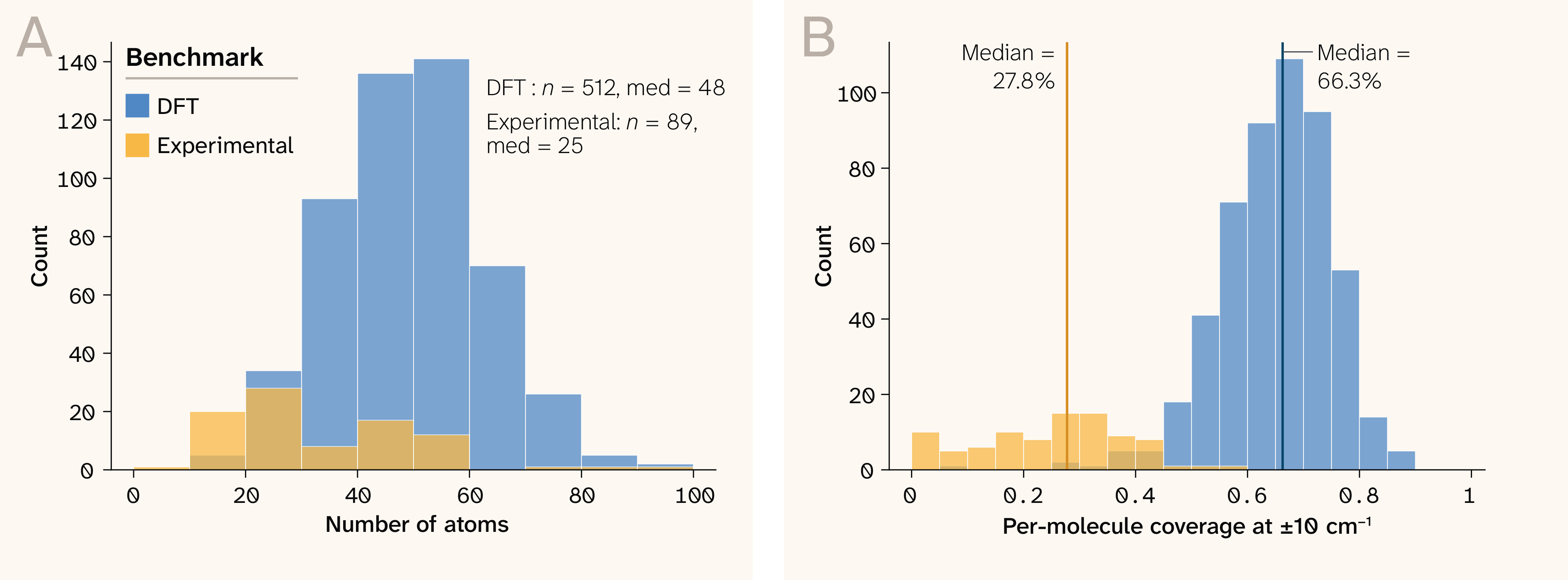
Figure 2. Test set composition.
(A) Distribution of molecule sizes (heavy-atom count) across the 1,000 DFT and 89 experimental molecules, binned in 10 heavy-atom increments. The DFT set is concentrated around 40–60 heavy atoms (median 48), while the experimental set skews smaller (median 25).
(B) Per-molecule coverage tolerance is set at 10 cm−1 for both benchmarks; DFT fingerprint coverage (median 67.2%) substantially exceeds experimental coverage (median 27.8%), consistent with the intensity calibration bottleneck described in the discussion section.
Metrics
The primary metric is coverage@δ: the fraction of reference modes with any predicted mode within ± δ cm−1 (nearest-neighbor recall, or Hungarian match). Intensity-weighted variants upweight strong reference modes. We report coverage at δ = 10 cm−1 and δ = 15 cm−1, the latter being the standard tolerance in ML-for-Raman work 33. Bootstrap 95% confidence intervals use the BCa method with 5,000 resamples. A secondary metric is weighted coverage@δ, which accounts for variation in intensity relative to the matched mode. Essentially, even if positions match to within δ cm−1, if the intensities fall outside an acceptable threshold relative to the reference intensity at that position, the mode isn't counted as a match.
Code, including model weights, training algorithms, and some components of our system, is available in this GitHub repo (DOI: 10.5281/zenodo.20329932).
The results
SpectraLoRA recovers two-thirds of fingerprint modes at DFT-level positional accuracy, zero-shot
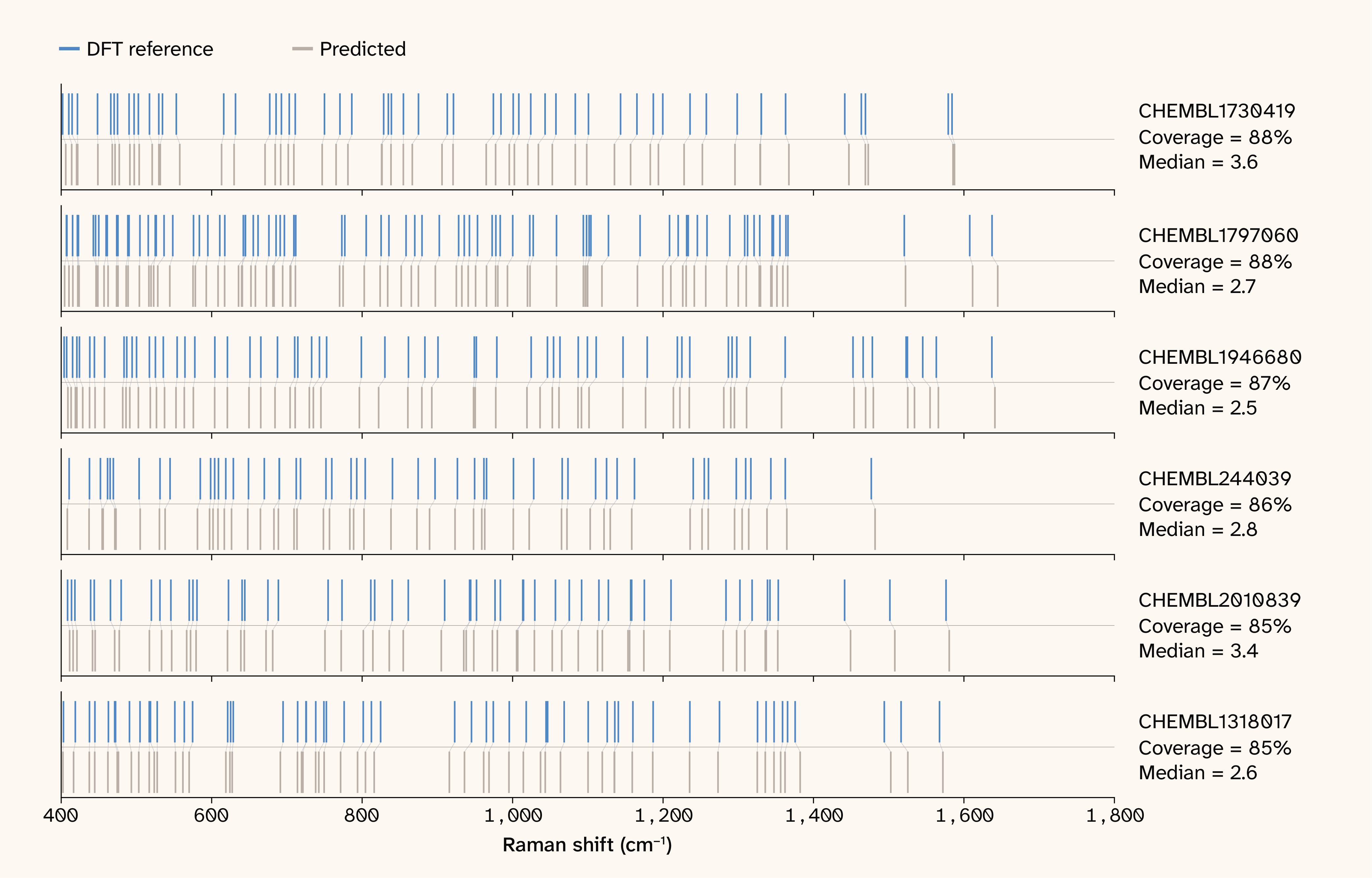
Figure 3. Barcode plot of Raman sticks DFT versus model prediction.
A plot showing the wavenumber differences between model predictions and DFT references. This plot shows strong alignment between the model-predicted wavenumber and reference data.
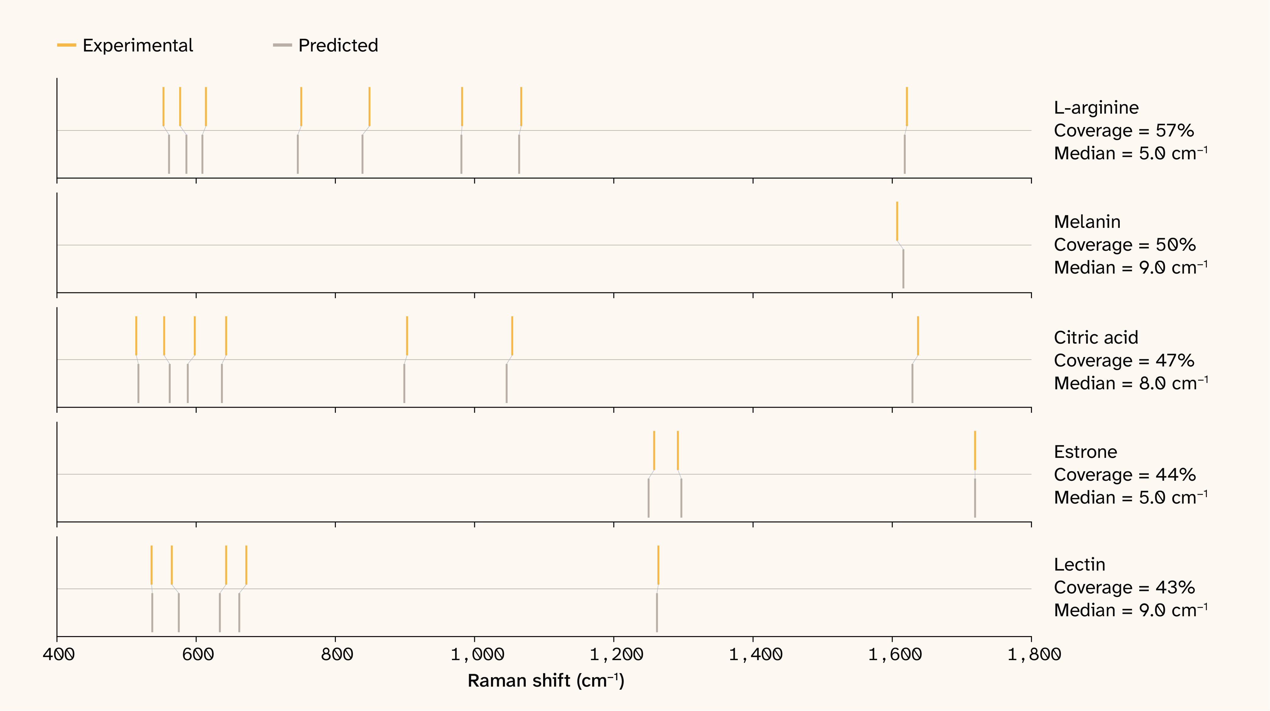
Figure 4. Raw lines wavenumber concordance.
Wavenumber differences between model predictions and experimentally determined references, showing strong alignment between the model-predicted wavenumber and reference data.
Figure 3 and Figure 4 show the raw lines predictions versus ground truth for simulated and experimental data. Table 1 and Figure 5 summarize the principal results. Overall, these results demonstrate that SpectraLoRA has learned to predict spectral peaks with a lower median error than the uncertainty of DFT, without being directly trained on Raman spectra. On the blind, entirely out-of-distribution DFT benchmark (1,000 Raman ChEMBL molecules absent from training), the model places 67.2% of reference modes in the fingerprint region for coverage@δ for δ = 10 cm−1, with 58.1% intensity-weighted coverage. Full-range coverage is 60.6% at ± 10 cm−1 and 68.7% at ± 15 cm−1. The matched-mode median error is 3.56 cm−1 (90th percentile: 8.27 cm−1), well below the ~10–20 cm−1 error of scaled DFT harmonic frequencies relative to experiment, meaning SpectraLoRA recovers DFT’s own answer to within a fraction of DFT’s inherent uncertainty.
| Benchmark | Region | Coverage@10 | Weighted coverage@10 | Median |
|---|---|---|---|---|
| DFT raw lines | Fingerprint | 0.672 | 0.581 | 3.04 |
| DFT raw lines | Full range | 0.606 | 0.332 | 3.56 |
| Experimental | Fingerprint | 0.269 | 0.215 | 5.00 |
Table 1. Zero-shot OOD evaluation on 1,000 Raman ChEMBL molecules (DFT) and 89 experimental spectra.
We trained the model on SPICE/NABLA2DFT/QM9/QM7, none of which contain Raman ChEMBL molecules or Raman-specific labels. Coverage is nearest-neighbor recall. Error statistics are over matched pairs at ± 10 cm−1. Intensity MAE is in log10 units. These results demonstrate zero-shot transfer to unseen larger peptides and experimental spectra.
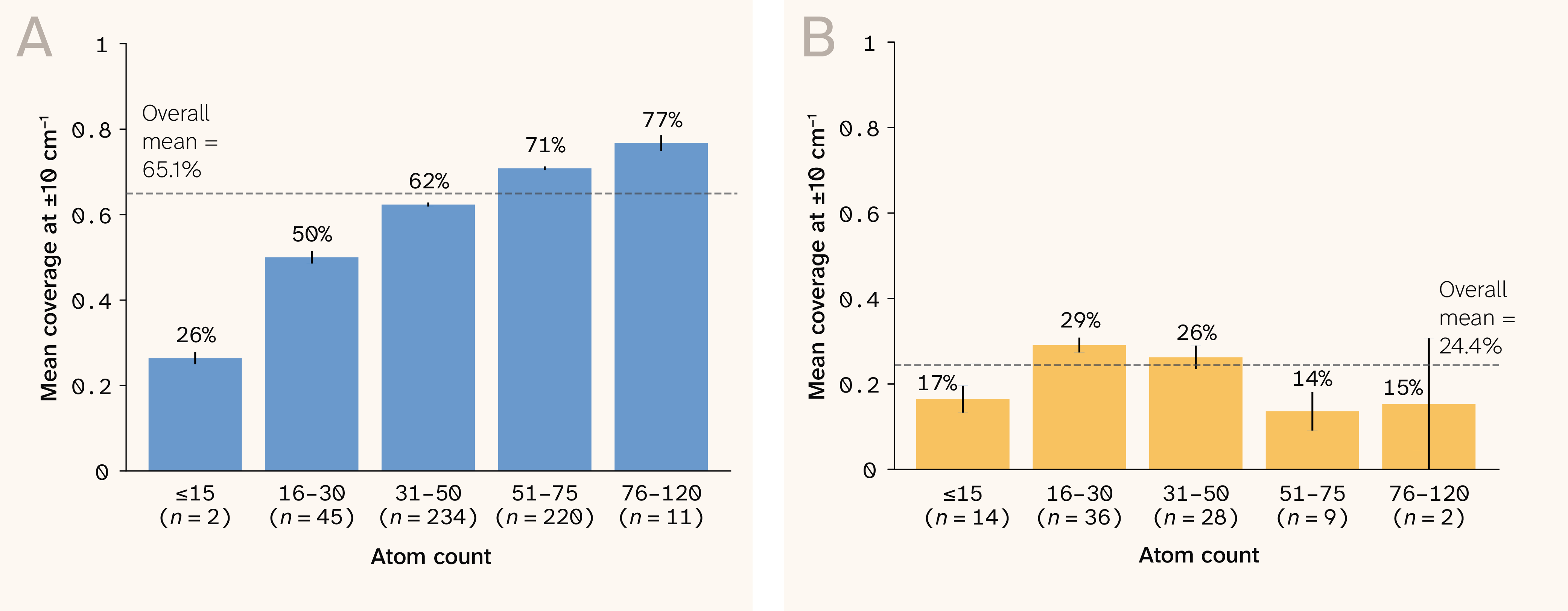
Figure 5. Zero-shot mode recovery.
(A) DFT mode recovery by molecule size, showing stable performance across the molecular weight and size ranges with a better performance for larger molecules.
(B) Experimental mode recovery by molecule size, showing lower but consistent coverage across size bins. Error bars denote standard error.
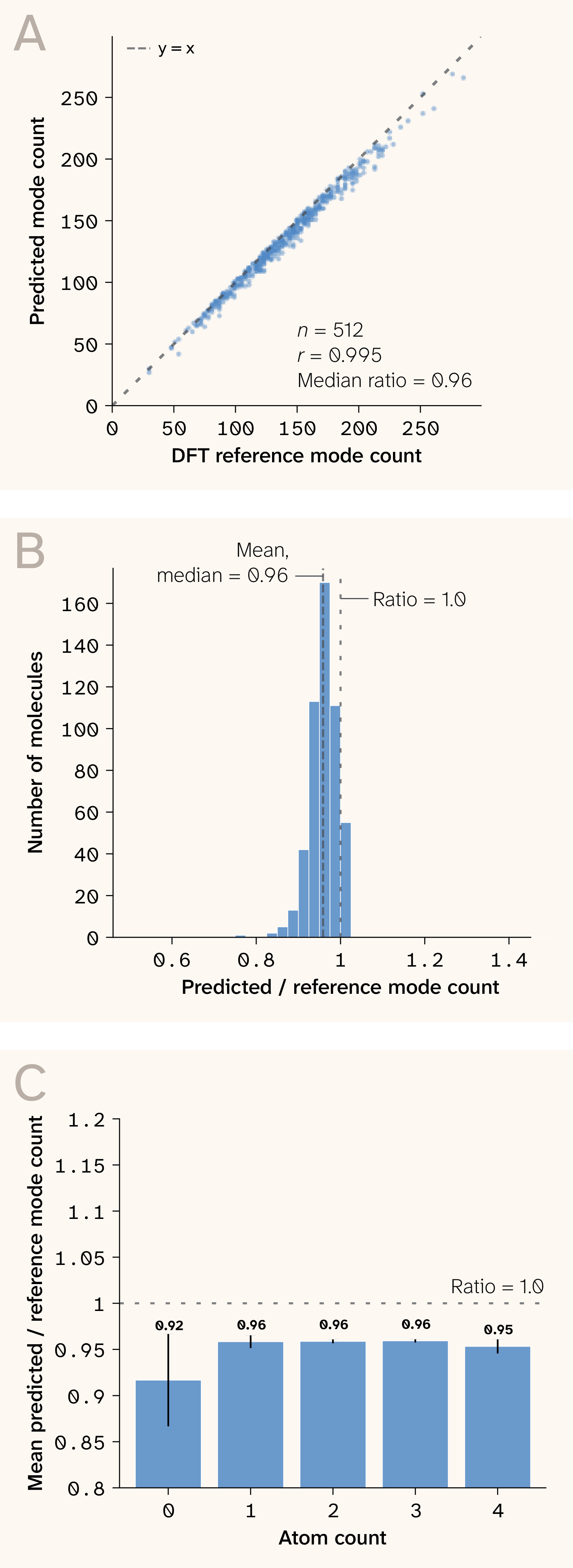
Figure 6. Mode count agreement between predicted and DFT reference spectra.
(A) Parity plot showing strong correlation (r = 0.995).
(B) Distribution of predicted/reference mode-count ratios (median 0.96).
(C) Ratio stability across molecule sizes.
The predicted-to-reference mode-count ratio is 0.96 (median; Pearson r = 0.995), confirming that the model produces approximately the correct number of vibrational modes without systematic suppression or inflation (Figure 6). Notably, we never trained the model on Raman spectra or vibrational labels of any kind — frequencies emerge from the learned Hessian via diagonalization and the chain rule, making this a physics-derived zero-shot prediction rather than a domain-transfer one.
We trained SpectraLoRA entirely on simulated DFT representations, so an open question is how well its predictions transfer to experimentally collected spectra. DFT assumes an isolated molecule, while experimental measurements capture environmental effects like motion due to temperature as well as instrument noise. We evaluated SpectraLoRA’s predictive performance on data from RamanBiolib 8, a small set of molecules with experimental Raman spectral measurements. When evaluated against 89 experimental Raman spectra, the model correctly places 26.9% of peaks within ± 10 cm−1, which is a large drop from the 67.2% accuracy on simulated data.
Figure 7 shows the signed residual distribution. It reveals a small but statistically significant negative bias: The median signed error is −2.5 cm−1 full-range (−2.22 cm−1 fingerprint), indicating the model slightly underpredicts vibrational frequencies. This bias is well within normal DFT error bounds (~0.25% at 1,000 cm−1) and is consistent with training on mixed-functional data, where the applied scaling factor of 0.967 doesn't perfectly absorb functional-dependent harmonic overestimation across all chemical environments.
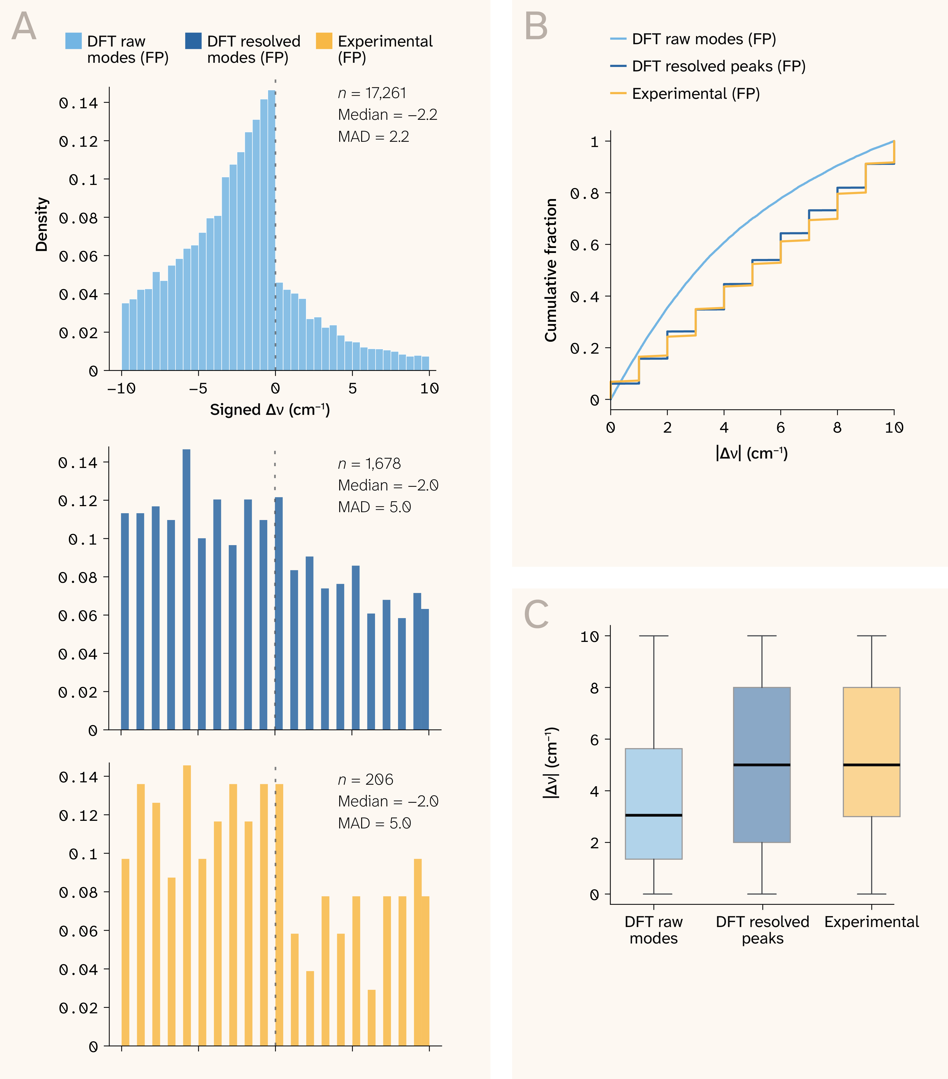
Figure 7. Mode-level frequency error across benchmarks (fingerprint region, 10 cm−1 tolerance).
(A) Signed error distribution for DFT raw modes (n = 17,261), DFT resolved peaks after broadening and peak extraction (n = 1,678), and experimental peaks (n = 206). The DFT raw-mode distribution shows a systematic negative bias of approximately 2.5 cm−1, consistent with imperfect scaling factor absorption across mixed-functional training data.
(B) Empirical CDF of absolute positional error, staircase appears due to the ECDF being fundamentally discontinuous, it changes only at observed values, and the number of observed values is small, thereby causing jumps. Roughly 80% of raw-mode matches fall within 5 cm−1. DFT resolved peaks and experimental peaks track closely, indicating that the dominant error is introduced at the peak formation stage, not at the DFT-to-experiment boundary.
(C) Per-benchmark boxplots of absolute error confirming tighter error distribution for raw modes relative to resolved and experimental peaks.
SpectraLoRA predicts peak locations better than spectral intensities
The principal limitation is intensity calibration. Intensity calibration errors are likely due to numerical errors arising from polarizability approximations during data calibration; however, this is only a hypothesis. Note, that the model training procedure does not involve directly predicting intensity. Matched-mode intensity MAE is 0.854 in log10 units on DFT raw lines, approximately a 7 × multiplicative error when compared to reference DFT intensity. This error implies that the predicted values in a.u. can be up to seven times off relative to a reference. This reflects the fundamental difficulty of predicting polarizability derivatives from equilibrium geometry 24, 34. After broadening and peak extraction, matched intensity MAE decreases to ~0.46 for both DFT peaks and experimental peaks, partly because peak extraction preferentially retains stronger, more predictable modes. Figure 8 shows the intensity scatter and Bland–Altman analysis: While the mean difference is near zero (−0.05), the limits of agreement (± 0.7 normalized) confirm high per-mode variance.
Expand to see Bland-Altman analysis for the full distribution of spectral intensity predictions and their errors or continue on for a summary of errors by wavenumber range in Figure 9.
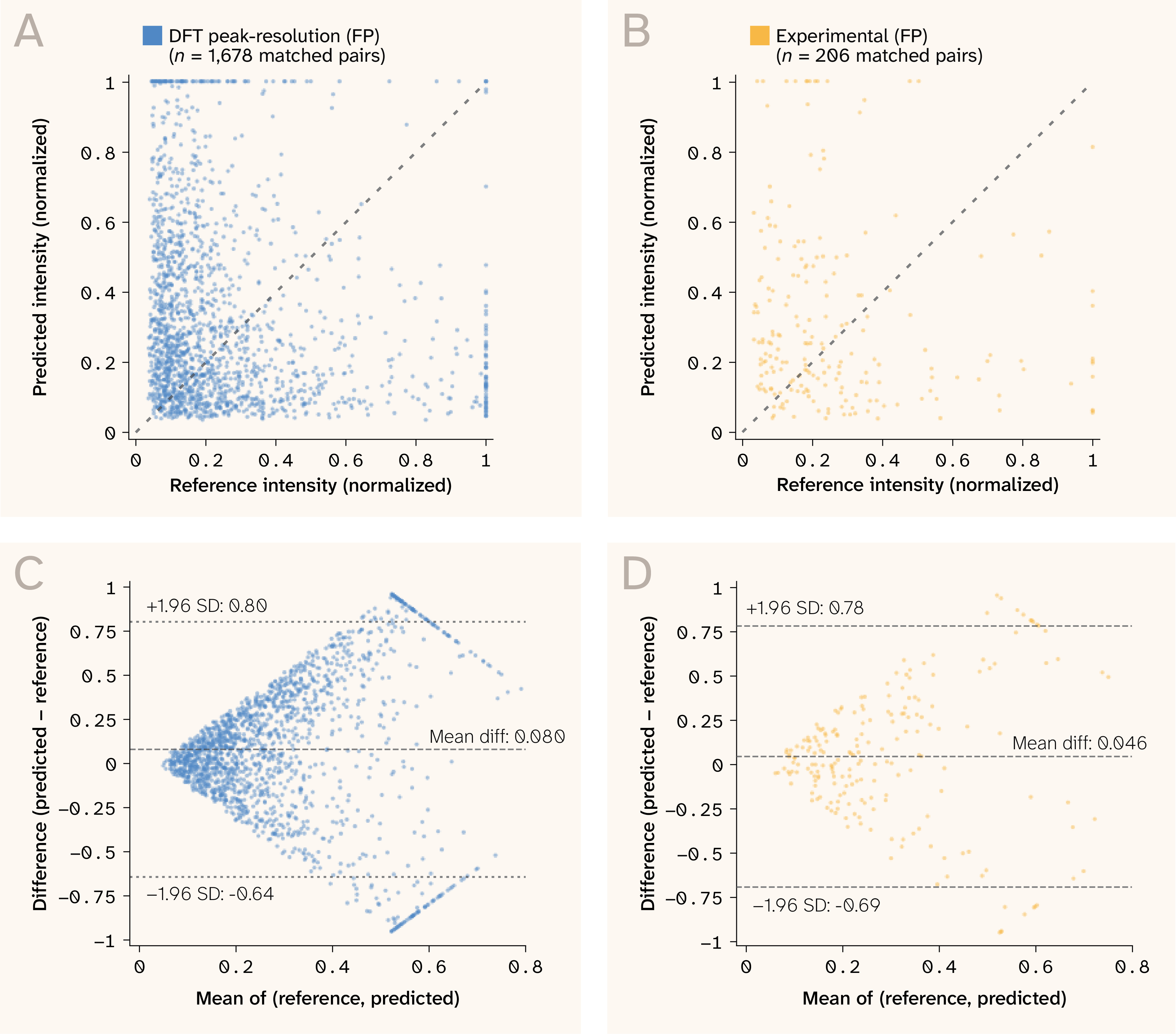
Figure 8. Intensity agreement for matched modes (fingerprint, ± 10 cm−1)
(A–B) Predicted vs. reference normalized intensity for DFT peaks (A, n = 1,678) and experimental peaks (B, n = 206).
(C–D) Bland–Altman plots showing near-zero mean difference but wide limits of agreement, consistent with ~7 × multiplicative error relative to DFT.
Prediction of peak locations is less accurate for experimental spectra
The 60.6% to 26.9% degradation from raw lines to DFT peaks to experimental peaks is explainable. We understand this degradation as follows. Discrepancies between calculated and experimental spectra emerge predominantly during the convolution of discrete DFT modes into broadened, resolved peaks, rather than at the raw computational boundary. This implicates intensity calibration and mode assignment as the limiting factors, rather than a systemic failure of the optimized structure. The mathematical broadening process, particularly when using a Voigt distribution, distributes signal into wide Lorentzian tails. As peaks merge, these underlying tails sum together, artificially inflating the apparent peak intensities and causing additive errors that compound across dense spectral regions 35.
Since the polarizability tensor is the primary factor in intensity prediction, and given we used DeePMD approximations of the polarizability tensor instead of full DFT computations, this is likely a source of error in intensity prediction. However, since the peak locations are somewhat accurate, the error in the intensity predictions could be mitigated by further training on a more appropriate distribution to incorporate experimental effects. The relatively worse intensity is not of as great a concern given our raw line metrics, and the application being screening. Within fingerprint sub-bands (Figure 9), the 400–800 cm−1 region shows the strongest weighted coverage (53.8%), while 1,200–1,600 cm−1 is weakest (16.9%).
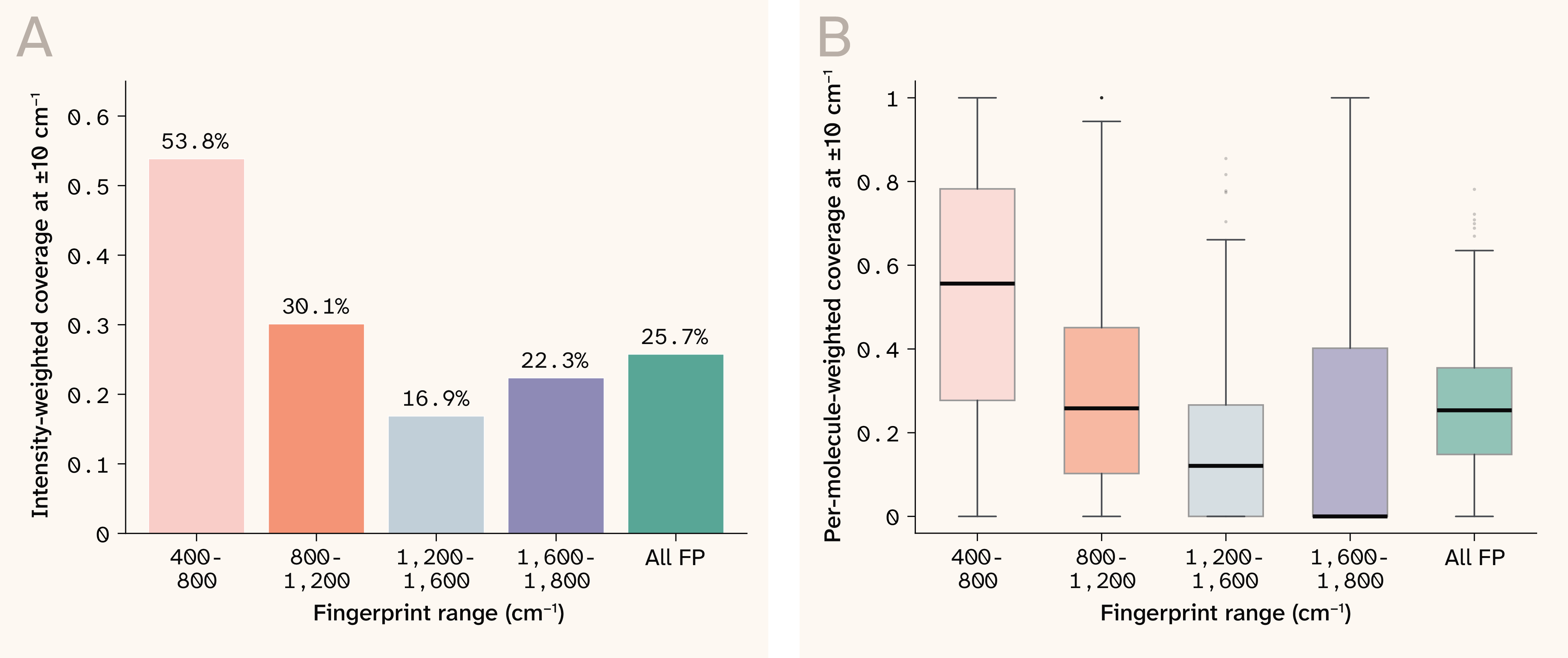
Figure 9. Fingerprint sub-band analysis (DFT peak-resolution benchmark, ± 10 cm−1)
(A) Intensity-weighted coverage by 400 cm−1 sub-band; the 400–800 cm−1 region (skeletal bending, ring deformations, etc.) is strongest, while 1,200–1,600 cm−1 (C=C stretching, aromatic modes, etc.) is weakest, reflecting domain shift from small-molecule training data.
(B) Per-molecule distribution of weighted coverage within each sub-band.
Per-molecule coverage when weighted by intensity shows a relatively consistent decline across fingerprint regions relative to unweighted coverage
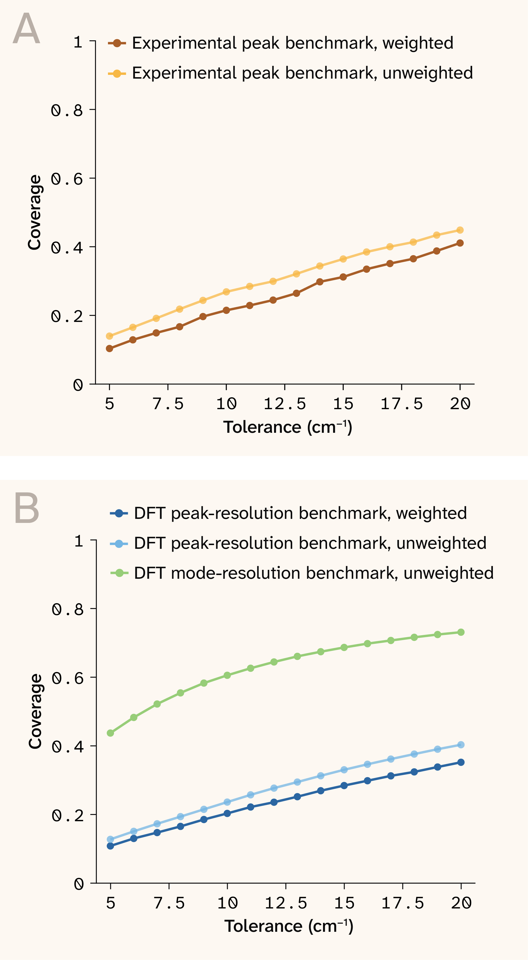
Figure 10. Coverage vs. tolerance window across benchmarks.
(A) Depicts experimental thresholds for both unweighted and weighted coverage.
(B) Depicts the DFT thresholds for both weighted and unweighted coverage.
The gap between raw-line (blue, “unweighted”) and peak-resolution (light blue, “weighted”) curves quantifies the loss introduced by broadening and peak extraction.
It's clear from Figure 9 that per-molecule coverage when weighted by intensity shows relative consistency across fingerprint regions. Consequently, we determine that the dominant loss in resolution occurs as a result of intensity calibration and broadening, not at the DFT-to-experiment boundary. In essence, when we isolate raw-line coverage and compare this to the noted drop in coverage when using intensity weighting, we can reasonably infer that differences in visual concordance between prediction and target are likely attributable to intensity-derived effects.
Prediction of spectral intensities is less accurate for experimental spectra
Median cosine similarity on broadened spectra is 0.218 (DFT, full range) and 0.192 (experimental, measured support). These are deliberately conservative: Cosine collapses frequency placement, intensity calibration, and peak merging into a single score. Figure 11 shows representative broadened spectral overlays, illustrating qualitative agreement in peak positions despite intensity miscalibration. The tolerance sweep (Figure 10) shows smooth improvement with wider windows, consistent with a model that localizes the correct vibrational neighborhoods before achieving exact peak resolution.
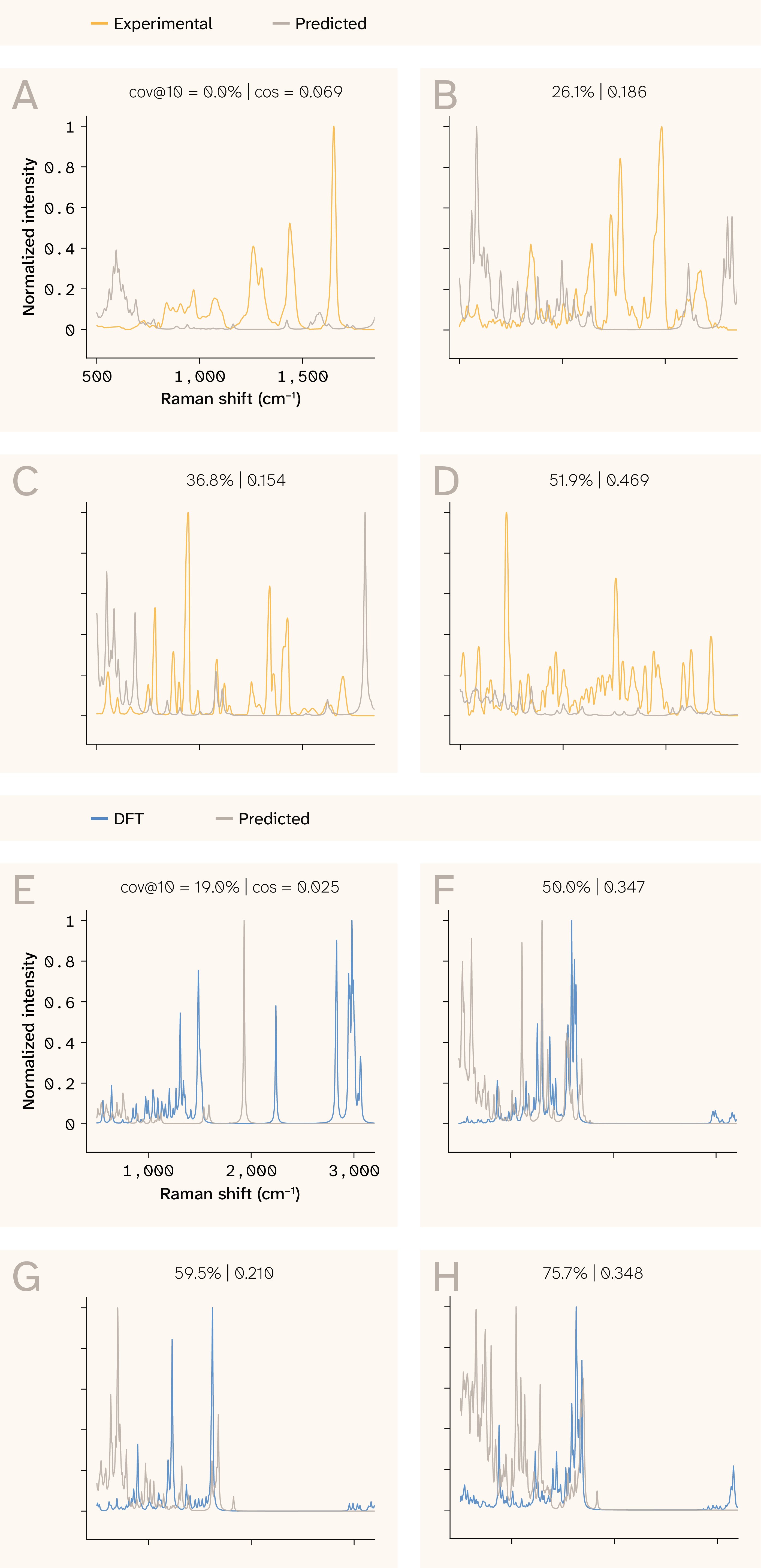
Figure 11. Broadened spectral overlays.
We depict a representative set of Raman spectra after ranking the molecules of the test set by the coverage@10 metric.
(A–D) Experimentally determined spectra relative to SpectraLoRA predictions:
(A) 0th percentile, (B) 20th percentile, (C) 40th percentile and (D) 60th percentile
(E–H) SpectraLoRA predictions relative to a DFT ground truth:
(E) 0th percentile, (F) 20th percentile, (G), 40th percentile, and (H) 60th percentile.
The molecules we selected are explicitly chosen to be uniform across all coverage levels. The distribution over coverages, however, is not uniform.
Predicted spectra (blue) are compared against DFT reference spectra (orange) after Lorentzian broadening (σ = 12 cm−1). The model captures the dominant peak positions while exhibiting characteristic intensity miscalibration.
Training an adapter network on experimental spectra improves intensity prediction
An analysis of the errors in intensity prediction as a function of wavenumber reveals regularities that we can exploit to improve intensity prediction. The fingerprint sub-band analysis (Figure 9) reveals that the 400–800 cm−1 region shows substantially stronger weighted coverage (53.8%) than the 1,200–1,600 cm−1 region (16.9%). This is not a random failure pattern: The 1,200–1,600 cm−1 range is dominated by C=C stretching, aromatic ring deformations, and C–N/C–O bending modes characteristic of drug-like organic molecules 23. These functional-group vibrations are heavily represented in the Raman ChEMBL evaluation set (fused heterocycles, sulfonamides, amide linkages), but underrepresented in the training data, which consists primarily of small molecules lacking such structural complexity. The sub-band performance drop is a predictable consequence of this domain shift rather than an architectural deficiency and could be mitigated by training on a subset of Raman ChEMBL.
Alignment results
Spectral refinement via evolution strategies
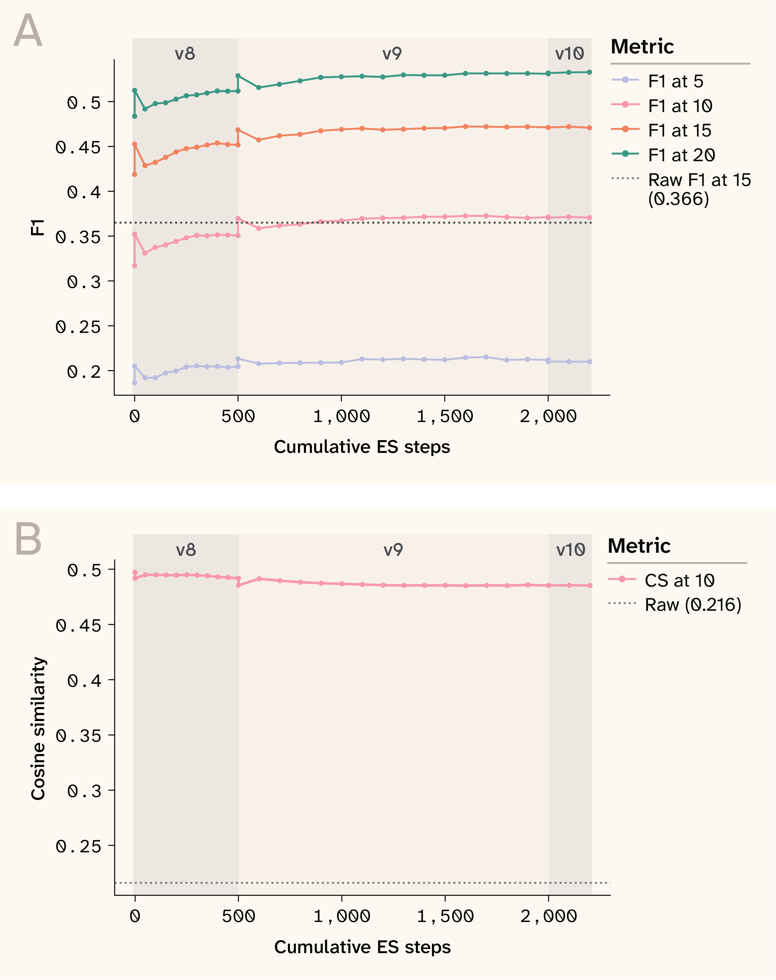
Figure 12. Convergence of evolution strategies.
(A) The result of the evolution strategy with respect to improving F1 at various wavenumber cutoffs as steps and stages increase.
(B) Consistent cosine similarity across ES stages.
Convergence of evolution strategies across ~2,000 cumulative steps. F1 at multiple tolerances improves monotonically in the fingerprint region. Version boundaries (v8 to v9 to v10) correspond to warm-start continuations with increased compute budget.
To bridge the gap between raw Hessian-derived spectral peak location predictions, which are reasonably accurate, and spectral intensity predictions, we train a post-hoc spectral refinement network: a 1D U-Net (447K parameters) with FiLM conditioning on Morgan fingerprints that learns a residual correction to the broadened predicted spectrum. Training proceeds in two phases. Phase 1 uses the peak-weighted RMSE loss of Sorrentino et al. 19, which improves fingerprint F1@15 from 0.426 to ~0.44. Phase 2 applies natural evolution strategies (NES) 20 to directly hill-climb the non-differentiable F1@15 metric. At each step, we apply K = 80 antithetic Gaussian perturbations to the decoder weights, evaluate F1@15 for each, and estimate the gradient from the reward-weighted perturbation directions. This black-box approach succeeds where differentiable surrogates (soft-F1, REINFORCE) failed in practice, because weight-space perturbations produce coherent spectral changes (peak shifts, intensity adjustments) rather than the unstructured noise that output-space exploration generates. That is, perturbing the model's weights by a small vector produces a smooth, coherent change in the output spectrum (peaks shift, intensities adjust), whereas methods that explore in output space (e.g., REINFORCE) encounter a piecewise-constant reward landscape where small spectral changes either leave F1 unchanged or cause discontinuous jumps as peaks appear or vanish. The training progress is summarized in Figure 12.
To ensure rigorous evaluation and prevent data leakage, we strictly partitioned the 1,000 OOD Raman ChEMBL molecules. We used a subset of 500 molecules as the optimization set for the phase 1 RMSE pre-training and phase 2 NES hill-climbing. We reserved a strictly sequestered, held-out set of 500 molecules for final evaluation. The metrics in Table 2 reflect the model’s performance solely on this held-out test split. To maximize large-molecule coverage, one can adopt a less difficult split, for instance, 80/20.
| Metric | Mol2Raman (in-dist QM9) | Baseline (OOD) | +ES refined (OOD) | Δ |
|---|---|---|---|---|
| FP F1@10 | 0.551 | 0.321 | 0.418 | +30% |
| FP F1@15 | 0.631 | 0.426 | 0.532 | +25% |
| FP F1@20 | 0.705 | 0.489 | 0.598 | +22% |
| FP Recall@15 | 0.634 | 0.438 | 0.703 | +60% |
| FP Precision@15 | 0.629 | 0.444 | 0.440 | −1% |
| Full F1@15 | — | 0.366 | 0.472 | +29% |
| Full F1@20 | — | 0.420 | 0.532 | +27% |
| Cosine (full) | 0.689 | 0.216 | 0.486 | +125% |
Table 2. Spectral refinement results.
Spectral refinement results (fingerprint region, 500–2,100 cm−1). Mol2Raman numbers are from Sorrentino et al. Table 2 (fingerprint) evaluated in-distribution on QM9 19. SpectraLoRA+ES is evaluated out-of-distribution on Raman ChEMBL. The comparison is not apples-to-apples, peak extraction parameters and chemical domains differ, but the recall advantage (0.703 vs. 0.634) is notable.
Table 2 reports the refined metrics alongside Mol2Raman 19 for context. The comparison isn't apples-to-apples: Mol2Raman is a SMILES-to-peak regressor that we've evaluated in-distribution on small QM9 molecules (≤ 9 heavy atoms, C/H/O/N/F), while we evaluate SpectraLoRA entirely out-of-distribution on drug-like molecules (median 24 heavy atoms, elements including S, Cl, Br, P). Peak extraction parameters also differ between the two systems. Nonetheless, the relative comparison is informative: SpectraLoRA+ES achieves 84% of Mol2Raman’s fingerprint F1@15 on a substantially harder benchmark, and exceeds Mol2Raman’s recall (0.703 vs. 0.634), indicating that the physics-based model finds more real peaks at the cost of lower precision. We didn't target the CH stretching region (2,800–3,200 cm−1) 36 by the refinement.
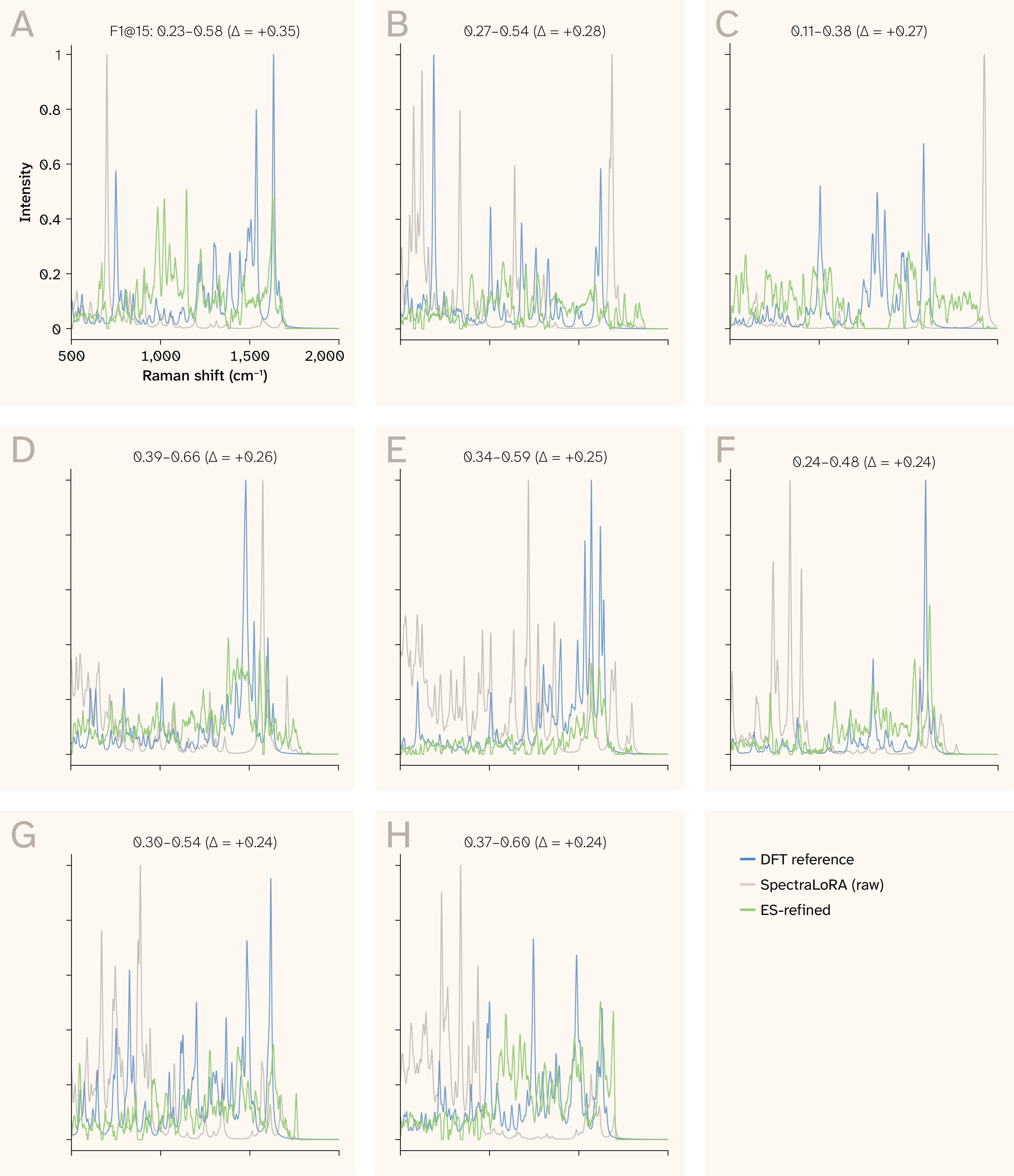
Figure 13. Network predictions vs. refined predictions.
The results of applying RefinementNet to the candidate SpectraLoRA intensity predictions for the eight most-improved molecules.
(A) The spectrum with the largest improvement after the application.
(B–H) The next largest improvements in descending order.
The baseline is DFT. The plots are chosen uniformly over all coverage levels. However, the coverage distribution is not uniform. Before/after spectral refinement for the top eight most-improved test molecules. Blue: DFT reference; gray: raw SpectraLoRA prediction; green: ES-refined output. The refinement suppresses spurious peaks, sharpens real peaks, and improves spectral alignment without changing peak positions by more than ~5 cm−1.
In Figure 13, the eight molecules with the largest improvement in F1 score after evolution strategy refinement are shown. Across all eight cases, the ES-refined spectra (green) track the DFT reference spectra (blue) more closely than the raw SpectraLoRA predictions (gray), with per-molecule F1 improvements (Δ) ranging from +0.24 to +0.26. The refinement network achieves these gains primarily by suppressing spurious predicted peaks that lack corresponding reference modes and by refining the intensities of true peaks, bringing the predicted spectral envelope into closer agreement with the reference. Importantly, the refinement preserves the underlying frequency positions predicted by the backbone, as peak shifts remain within 5 cm−1, indicating that the U-Net correction operates on intensity and shape rather than relocating vibrational modes. The consistency of the improvement across molecules of varying spectral complexity suggests that the evolution strategy optimization generalizes across chemical environments rather than overfitting to a narrow subset of the training distribution.
Next steps and feedback
The precision gap (0.440 vs. Mol2Raman’s 0.629) suggests that mode selection is the primary remaining bottleneck: The model predicts too many spectroscopically weak peaks that survive broadening. A dedicated mode-filtering head trained with DFT Raman activity supervision would directly address this. Better polarizability prediction, via explicit electron-density modeling or higher-order derivative targets, would address the underlying intensity bottleneck. Multi-fidelity training incorporating both DFT references and experimental spectra, and extension to peptides and proteins, are natural follow-ons. Others may want to develop a decoder or network that takes as input the predicted Raman spectra and attempts to infer molecular properties.
Please share comments with any observations about how we could improve the scope or performance of SpectraLoRA.
Try the model! To apply SpectraLoRA to your own work, review the demo here.
Conclusion
SpectraLoRA demonstrates that a 22.5M-parameter equivariant molecular GNN model, adapted via parameter-efficient fine-tuning and alignment, can serve as a high-throughput surrogate for DFT dynamical matrices. On a blind, out-of-distribution benchmark of 1,000 drug-like molecules, spanning elements and structural motifs absent from training, the model recovers 60.6% of vibrational modes within ± 10 cm−1 with median positional error of 3.56 cm−1, sufficient for thermochemical applications at linear cost. A post-hoc spectral refinement stage, combining peak-weighted RMSE pre-training with evolution strategies for direct F1 optimization, pushes fingerprint F1@15 from 0.426 to 0.532 and achieves 70.3% peak recall, exceeding the in-distribution recall of the end-to-end Mol2Raman baseline on a substantially harder chemical domain. The precision gap (0.440 vs. 0.629) shows that mode selection should be the specific target for future work.
This framework demonstrates that we can approximate modes well in silico, even for large peptides, using post-training techniques. Therefore, scalable compound screening is entirely possible. To better approximate the actual intensities, alignment and reinforcement learning-based strategies show promise in correcting shape. This provides a clear framework for eventually matching experimental measurement in silico. The key limitation is the amount of experimental data available to calibrate this model. Distribution shift isn't as much of a concern given the results presented — namely, that our model performs reasonably well, not only on a test set that's held out, but on one that's drawn from an entirely different distribution over more complex molecules. The field can, therefore, simply post-train and align reasonably to close the simulation-to-reality gap as it applies to Raman spectroscopy.
Be the first to comment on this publication.